Gradient Descent

Most functions you want to minimize in machine learning do not have a closed-form solution. You cannot just set the gradient to zero and solve like you do with linear regression. Instead, you start somewhere random and take small steps downhill, using the gradient as your compass. This is gradient descent.

\[\theta_{k+1} = \theta_k - \alpha \nabla f(\theta_k)\]

You have a function $f: \mathbb{R}^d \to \mathbb{R}$ (the loss), parameters $\theta \in \mathbb{R}^d$, and a learning rate $\alpha > 0$. At each step you compute the gradient $\nabla f(\theta_k)$, which points uphill, and move opposite to it.

Intuition: “You are standing on a foggy mountain. You cannot see the whole terrain, but you can feel the slope under your feet. To get to the valley, you step in the direction where the ground drops the most. The learning rate $\alpha$ is how big a step you take: too small and you never get there, too large and you stumble past the valley and have to turn back.”

The Learning Rate

The learning rate $\alpha$ is the single most important hyperparameter. A small $\alpha$ means reliable but slow progress. A large $\alpha$ means fast progress but risk of overshooting.

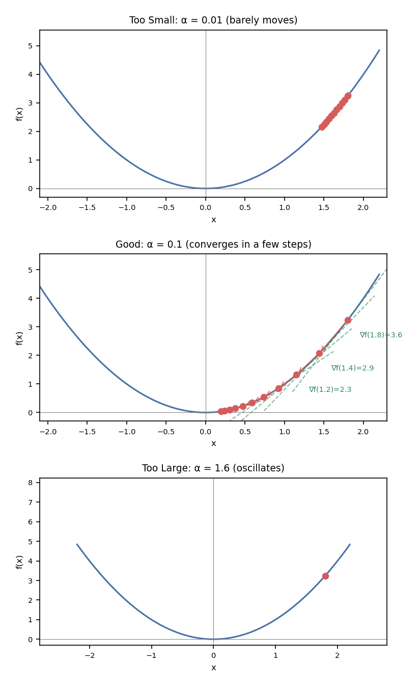
For the simple function $f(x) = x^2$ starting at $x = 1.8$:

• Too small ($\alpha = 0.01$): each step barely moves. You will reach the minimum eventually, but it takes hundreds of steps.
• Good ($\alpha = 0.1$): the steps shrink naturally as the gradient gets smaller near the minimum. You converge in 5-10 steps.
• Too large ($\alpha = 1.6$): the step overshoots past the minimum, and the next step overshoots back. You oscillate and may never settle.

Intuition: “The learning rate determines how much you trust each gradient measurement. A small rate is cautious but slow. A large rate is aggressive but unstable. The sweet spot depends on the curvature of your loss surface: flatter surfaces can handle larger rates.”

GD on a 2D Surface

Real problems have more than one parameter. The gradient is a vector, and each component tells you the slope along that parameter’s axis.

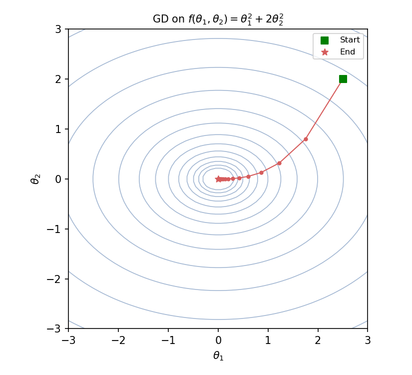
This is $f(\theta_1, \theta_2) = \theta_1^2 + 2\theta_2^2$, an elliptic paraboloid. The gradient is $\nabla f = [2\theta_1, 4\theta_2]^\mathsf{T}$. Because the surface is steeper along $\theta_2$ (coefficient 2 vs 1), GD takes bigger steps in that direction at first, then zig-zags as it approaches the minimum.

Intuition: “The gradient tells you the slope in every direction at once. You take a single step that combines all those directions. If one direction is steeper, you move more in that direction. This is why GD naturally follows the steepest path down, which is not always a straight line to the minimum.”

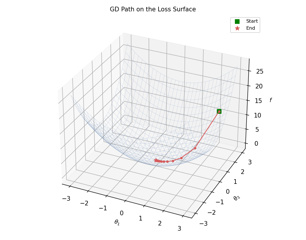
The 3D view makes it clear: the path starts on the steep wall, drops quickly into the valley, then follows the valley floor to the minimum.

Connection to Linear Regression

From the linear regression post, the loss is $L(\theta) = |X\theta - y|_2^2$ with gradient $\nabla L = 2X^T(X\theta - y)$. The exact solution via normal equations costs $O(nd^2 + d^3)$. Each gradient descent step costs $O(nd)$.

The tradeoff is:

• Exact solve (normal equations / QR): one shot, $O(nd^2 + d^3)$. Best for small $d$ (under a few thousand).
• Gradient descent: iterative, $O(nd)$ per step. Best for large $d$ (millions of parameters). You never form the $d \times d$ matrix $X^T X$.

This is the fundamental reason gradient descent dominates modern deep learning: models have millions of parameters, and forming a $10^6 \times 10^6$ matrix is not feasible.

Batch vs SGD vs Mini-Batch

The gradient $\nabla L = 2X^T(X\theta - y)$ uses all $n$ data points. This is batch gradient descent: accurate but expensive per step.

SGD (Stochastic Gradient Descent) approximates the gradient using a single randomly-chosen data point $i$:

\[\nabla L_i(\theta) = 2x_i^T(x_i^T\theta - y_i) \quad \text{where} \quad \mathbb{E}[\nabla L_i] = \nabla L\]

The gradient estimate is noisy but unbiased. Each step costs $O(d)$ instead of $O(nd)$, and the noise can actually help escape shallow local minima.

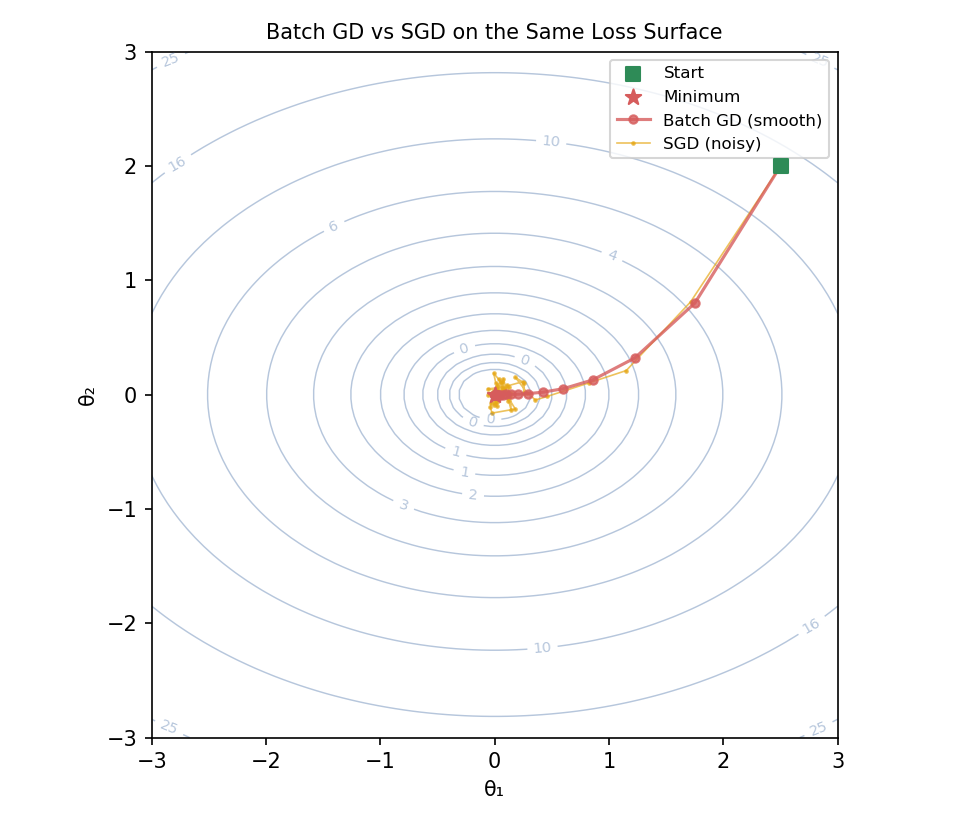
Mini-batch GD is the practical middle ground: use 32-1024 random points per step. Noisy enough to generalize, cheap enough to be fast, and easy to parallelize on GPUs. This is what every practical deep learning system uses.

Intuition: “Batch GD is like surveying the entire mountain before each step: accurate but slow. SGD is like glancing at one random pebble under your foot: noisy but fast. Mini-batch is like looking at a small patch of ground around you: good enough to make progress, fast enough to keep moving.”

Components

• $\theta \in \mathbb{R}^d$: parameters being optimized (weights of a model).
• $f: \mathbb{R}^d \to \mathbb{R}$: loss function, a scalar measure of how bad the current parameters are.
• $\nabla f(\theta) \in \mathbb{R}^d$: gradient of $f$ at $\theta$. Vector of partial derivatives, one per parameter.
• $\alpha$: learning rate. Step size. The most important hyperparameter to tune.
• $n$: number of data points (batch size for batch GD, 1 for SGD, $b$ for mini-batch).

Quick Reference

Aspect	Batch GD	SGD	Mini-Batch
Gradient estimate	Exact (all data)	Noisy (one point)	Moderate ($b$ points)
Cost per step	$O(nd)$	$O(d)$	$O(bd)$
Convergence	Smooth, monotonic	Bounces around minimum	Semi-smooth
Use case	Small $n$, convex problems	Very large $n$, escape local minima	Every practical system

Notes

• Gradient descent only guarantees convergence to a local minimum for convex functions. In deep learning, the loss surface is highly non-convex, but GD with mini-batches consistently finds solutions that generalize well.
• Momentum (Polyak, 1964) improves GD by adding a fraction of the previous update: $\theta_{k+1} = \theta_k - \alpha \nabla f(\theta_k) + \beta(\theta_k - \theta_{k-1})$. This smooths out oscillations and accelerates through flat regions.
• Adam (Kingma & Ba, 2015) combines momentum with per-parameter adaptive learning rates using estimates of first and second moments of the gradient. It is the default optimizer for most deep learning.
• The directional derivative (notation page) gives the mathematical foundation: $D_v f(\theta) = \nabla f(\theta) \cdot v$ is the slope along direction $v$. The negative gradient gives the steepest descent direction because it maximizes $\lvert \nabla f \cdot v \rvert$ among all unit vectors $v$.
• Learning rate schedules (step decay, cosine annealing, warmup) are essential in practice. Start with a small rate, increase it during warmup, then decay it as training progresses.