Backpropagation
A feed-forward network has thousands to trillions of parameters. Training it means computing the gradient of the loss with respect to every weight and bias, then using gradient descent to update them. Computing each gradient individually with finite differences would cost $O(P^2)$ for $P$ parameters: not feasible. Backpropagation computes all $P$ gradients in $O(P)$ total, using the chain rule and cached intermediate values.
This post walks through backprop on a two-layer FFN, step by step. The same pattern applies to any differentiable computation graph: convolutions, attention, transformers.
The Chain Rule (Refresher)
For scalar functions, the chain rule says:
\[\frac{dz}{dx} = \frac{dz}{dy} \cdot \frac{dy}{dx}\]For vector functions $f: \mathbb{R}^n \to \mathbb{R}^m$ and $g: \mathbb{R}^m \to \mathbb{R}^o$, the Jacobian form is:
\[J_{f \circ g}(x) = J_f(g(x)) \cdot J_g(x) \in \mathbb{R}^{o \times n}\]Each entry $(i, j)$ of the product is $\sum_k \frac{\partial f_i}{\partial g_k} \cdot \frac{\partial g_k}{\partial x_j}$: the chain rule summed over the intermediate dimension $k$. This is the mathematical basis of backprop: multiply Jacobians from the output to each parameter, reusing intermediate products.
Forward Pass: The 2-Layer FFN
Use the same two-layer FFN from the feed-forward networks post. Input $x \in \mathbb{R}^d$, hidden width $h$, output dimension $o$:
\[\begin{aligned} z_1 &= W_1 x + b_1, \qquad &W_1 \in \mathbb{R}^{h \times d}, \; b_1 \in \mathbb{R}^h \\ a_1 &= \sigma(z_1), \qquad &\sigma = \text{ReLU} \\ z_2 &= W_2 a_1 + b_2, \qquad &W_2 \in \mathbb{R}^{o \times h}, \; b_2 \in \mathbb{R}^o \\ \hat{y} &= z_2 \\ L &= \|\hat{y} - y\|_2^2 \end{aligned}\]The forward pass computes each step in order and caches the intermediate values $z_1$, $a_1$, $z_2$ (they will be needed during the backward pass). Without caching, the backward pass would have to recompute every intermediate, doubling the total cost.
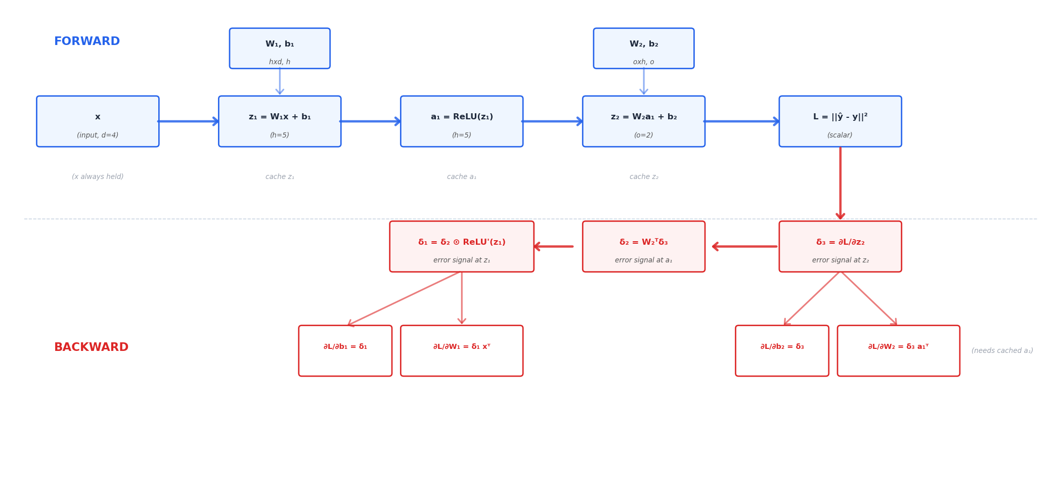
Backward Pass
Start at the loss $L$ and walk backward through each operation, computing the gradient of $L$ with respect to each intermediate and each parameter.
Step 1: Output gradient
\[\frac{\partial L}{\partial \hat{y}} = \frac{\partial L}{\partial z_2} = 2(\hat{y} - y) \in \mathbb{R}^o\]This is the “error signal” that will propagate backward.
Step 2: Output layer ($z_2 = W_2 a_1 + b_2$)
Given $\frac{\partial L}{\partial z_2}$, compute gradients for $W_2$ and $b_2$, plus the error signal for $a_1$:
\[\frac{\partial L}{\partial W_2} = \frac{\partial L}{\partial z_2} \cdot a_1^\mathsf{T} \in \mathbb{R}^{o \times h}, \qquad \frac{\partial L}{\partial b_2} = \frac{\partial L}{\partial z_2} \in \mathbb{R}^o\] \[\frac{\partial L}{\partial a_1} = W_2^\mathsf{T} \cdot \frac{\partial L}{\partial z_2} \in \mathbb{R}^h\]Each entry $(i, j)$ of $\partial L / \partial W_2$ is $\frac{\partial L}{\partial z_2}_i \cdot (a_1)_j$: the error for output $i$ multiplied by the activation of hidden unit $j$. If hidden unit $j$ was never active, $(a_1)_j = 0$, and its weights get zero gradient.
Intuition: “The gradient of a weight is the product of two things: the error signal from above and the input that fed into it from below. This is a rank-1 update: outer product of error and activation.”
Step 3: Activation ($a_1 = \sigma(z_1)$)
Pass the error signal through the activation derivative:
\[\frac{\partial L}{\partial z_1} = \frac{\partial L}{\partial a_1} \odot \sigma'(z_1) \in \mathbb{R}^h\]For ReLU, $\sigma’(z) = 1$ if $z > 0$, $0$ otherwise. If $z_1$ was negative during the forward pass, $\sigma’(z_1) = 0$ and the error signal is completely blocked: this is the “dead ReLU” problem.
Intuition: “The activation derivative acts as a gate. If $\sigma’(z) \approx 0$, the error signal cannot pass through and the gradient for everything below is zero. Smooth activations like GeLU and SiLU keep this gate open for all inputs.”
Step 4: Hidden layer ($z_1 = W_1 x + b_1$)
Same pattern as step 2, using $x$ as the input:
\[\frac{\partial L}{\partial W_1} = \frac{\partial L}{\partial z_1} \cdot x^\mathsf{T} \in \mathbb{R}^{h \times d}, \qquad \frac{\partial L}{\partial b_1} = \frac{\partial L}{\partial z_1} \in \mathbb{R}^h\]Step 5: Update with gradient descent
Now we have all four gradients: $\partial L / \partial W_1$, $\partial L / \partial b_1$, $\partial L / \partial W_2$, $\partial L / \partial b_2$. Use the gradient descent update from the GD post:
\[W_1 \leftarrow W_1 - \alpha \frac{\partial L}{\partial W_1}, \quad b_1 \leftarrow b_1 - \alpha \frac{\partial L}{\partial b_1}\]and the same for $W_2$, $b_2$.
The Full Chain Rule in One Expression
Writing the entire chain from $L$ to $W_1$ as a single product:
\[\frac{\partial L}{\partial W_1} = \frac{\partial L}{\partial \hat{y}} \cdot \frac{\partial \hat{y}}{\partial z_2} \cdot \frac{\partial z_2}{\partial a_1} \cdot \frac{\partial a_1}{\partial z_1} \cdot \frac{\partial z_1}{\partial W_1}\]Each “$\cdot$” is a Jacobian multiplication. Backprop computes this product from right to left, one factor at a time. The intermediate products ($\partial L / \partial z_2$, $\partial L / \partial a_1$, $\partial L / \partial z_1$) are cached and reused for multiple parameters at the same level, which is why the total cost is $O(P)$ and not $O(P^2)$.
Why Activation Functions Matter
The derivative $\sigma’(z)$ determines how much of the error signal reaches the layers below.
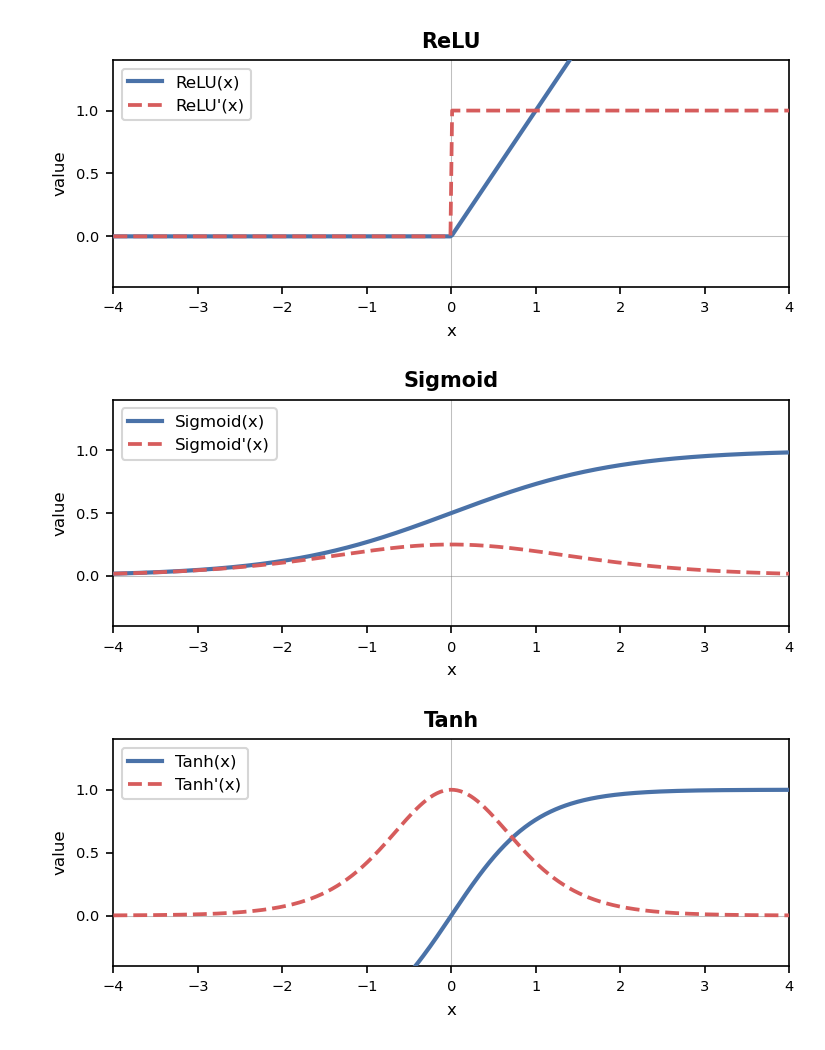
- ReLU has a hard kink at $x=0$ where the derivative jumps from 0 to 1. The derivative is 0 for $x < 0$, meaning any neuron with a negative pre-activation completely blocks gradient flow. Once many neurons are “dead”, the network stops learning.
-
Sigmoid has a smooth bell-shaped derivative. For large $ x $, the derivative is close to 0, causing vanishing gradients in deep networks. - Tanh has the same saturation problem as sigmoid. Its derivative peaks at $x=0$ and decays to 0 at the extremes.
This is why modern networks use ReLU (or its smooth variants GeLU/SiLU): the derivative is 1 for positive inputs, giving a clean gradient signal through most of the network.
Components
- $L$: loss function. A scalar that measures how wrong the prediction is.
- $\hat{y}$: prediction (output of the forward pass).
- $z_\ell$: pre-activation at layer $\ell$ (before the non-linearity).
- $a_\ell$: activation at layer $\ell$ (after the non-linearity).
- $W_\ell$, $b_\ell$: weights and biases at layer $\ell$. The parameters we want gradients for.
- $\sigma$: activation function, applied element-wise.
- $\partial L / \partial \cdot$: gradient of $L$ with respect to some tensor. These flow backward through the graph.
Quick Reference
| Operation | Forward | Backward (local gradient) |
|---|---|---|
| Linear $z = Wx + b$ | $z = Wx + b$ | $\partial L/\partial W = \delta \cdot x^\mathsf{T}$, $\partial L/\partial b = \delta$, $\partial L/\partial x = W^\mathsf{T} \cdot \delta$ |
| Activation $a = \sigma(z)$ | $a = \sigma(z)$ | $\partial L/\partial z = \partial L/\partial a \odot \sigma’(z)$ |
| Loss $L = |\hat{y} - y|^2$ | $L = |\hat{y} - y|^2$ | $\partial L/\partial \hat{y} = 2(\hat{y} - y)$ |
Notes
- The total cost of backprop is approximately $2\times$ the forward pass cost. Each parameter gets used once in the forward direction and once in the backward direction.
- Memory is the real bottleneck: all cached intermediates ($z_1$, $a_1$, $z_2$) must be stored until the backward pass finishes. This is why large models use gradient checkpointing (recompute some intermediates instead of storing them).
- Modern frameworks (PyTorch, JAX) implement automatic differentiation: you define the forward pass and the framework traces the computation graph, then builds the backward pass automatically. The gradient formulas are exactly the ones derived above.
- The same chain rule pattern applies to any architecture: convolutions, attention, skip connections. Each operation defines a forward function and a backward “gradient function” that multiplies the incoming error by the local Jacobian transpose.
- Skip connections (residual networks) help gradient flow by providing a path where the Jacobian is the identity matrix, so the error signal bypasses the activation derivative entirely.
Small Authors Note: I was quite demotivated during this semester… and my grades suffered, I didn’t score any internships, I had concerning symptoms from chronic intestinal ulcers, and I was unable to keep this blog going. With summer here, I am no longer pursuing corporate work for the time being. I will focus on self development, personal projects, life style improvements, and this blog will take a shift. This post was half-written, I have finished it and it will be followed by one of my greatest accomplishments, a PR on flashinfer (maintainers haven’t noticed it yet, but I’m still proud of myself). I have a large backlog of writing, that I need to format (I will likely be taking help from opencode’s generous deepseek v4 flash access). I will cover some more ML topics (FFN, MoE, etc.). And generally document my journey towards becoming a better developer and researcher. Hopefully I find sustainable employment in the future, due to these efforts.