<?xml version="1.0" encoding="utf-8"?><feed xmlns="http://www.w3.org/2005/Atom" ><generator uri="https://jekyllrb.com/" version="3.10.0">Jekyll</generator><link href="https://ahmadsaeedzaidi.github.io/feed.xml" rel="self" type="application/atom+xml" /><link href="https://ahmadsaeedzaidi.github.io/" rel="alternate" type="text/html" /><updated>2026-07-01T13:43:49+00:00</updated><id>https://ahmadsaeedzaidi.github.io/feed.xml</id><title type="html">Ahmad Saeed’s Dev Blog</title><subtitle>ML &amp; MLSys blog and notes</subtitle><author><name>Ahmad Saeed Zaidi</name></author><entry><title type="html">Flash Attention 2</title><link href="https://ahmadsaeedzaidi.github.io/flash-attention-2/" rel="alternate" type="text/html" title="Flash Attention 2" /><published>2026-07-01T00:00:00+00:00</published><updated>2026-07-01T00:00:00+00:00</updated><id>https://ahmadsaeedzaidi.github.io/flash-attention-2</id><content type="html" xml:base="https://ahmadsaeedzaidi.github.io/flash-attention-2/"><![CDATA[<h2 id="flash-attention-2">Flash Attention 2</h2>

<p>Replaces the standard attention $O = \text{softmax}(QK^T)V$ (which materializes a full $N \times N$ attention matrix in HBM) with an IO-aware tiled algorithm that streams Q, K, V through on-chip SRAM and never writes the $N \times N$ matrix out.</p>

<p>Motivation: standard attention is bottlenecked by memory, not FLOPs. For a sequence of length $N$ with head dim $d$, the $N \times N$ softmax matrix costs $O(N^2)$ memory and forces $O(N^2)$ HBM reads/writes on GPU. Flash Attention 2 cuts this to $O(N)$ HBM accesses (linear in sequence length) by recomputing attention in tiles and using the online softmax trick to merge partial results.</p>
<h2 id="standard-attention">Standard Attention</h2>

\[S = QK^T \in R^{N \times N}, \qquad P = Softmax_{row}(S) \in R^{N \times N}, \qquad O = PV \in R^{N \times d}\]

<h3 id="components">Components</h3>

<ul>
  <li>$Q, K, V \in R^{N \times d}$: query, key, value matrices for a single attention head, where $N$ is sequence length and $d$ is head dimension.</li>
  <li>$S \in R^{N \times N}$: attention scores, one scalar per (query, key) pair.</li>
  <li>$P \in R^{N \times N}$: attention weights after row-wise softmax. Each row sums to 1.</li>
  <li>$O \in R^{N \times d}$: output, one $d$-dim vector per query.</li>
</ul>

<h3 id="why-this-is-inefficient">Why this is inefficient</h3>

<ul>
  <li>
    <p><strong>Quadratic Memory Scaling $O(N^2)$:</strong> $S$ and $P$ are $N \times N$. For $N = 8192$ and fp16 that’s $8192^2 \cdot 2\text{B} \approx 128\text{ MB}$ per head, per layer. With 32 layers and 32 heads, this is already enormous amounts of memory. Since N is our sequence length, our memory scales quadratically in longer conversations, which is the main bottleneck for long-context LLMs.</p>
  </li>
  <li>
    <p><strong>Bandwidth bound $O(N^2)$:</strong> the GPU makes 3 trips to HBM.</p>
    <ol>
      <li>Read $Q, K$ to compute $S$. Write $S$ back to HBM.</li>
      <li>Read $S$ from HBM to compute the row-max for softmax, then write $P$ back.</li>
      <li>Read $P$ again to multiply with $V$. Three full passes over an $N \times N$ matrix that mostly lives in slow HBM, not fast SRAM.</li>
    </ol>

    <p>HBM might higher bandwidth than VRAM, but it’s still nothing compared to on-chip SRAM. We want to minimize HBM trips.</p>
  </li>
</ul>

<h2 id="flash-attention-2-1">Flash Attention 2:</h2>

<p>Break down the Q, K, V matrices into tiles that fit in SRAM, and compute attention block by block.</p>

<p>for now, we will assume a tile has size $m_r \times m_c$, where $m_r$ is the number of rows of Q, V and $m_c$ is the number of rows of $K^T$. This size is dynamically computed based on SRAM in the hardware, during compilation.</p>

<p>The full forward pass for a single Q block $Q_i$ loops over all K, V blocks $(K_j, V_j)$ where $K_j$ and $V_j$ are matrices of size $B_c \times d$, $B_r \times d$ respectively and accumulates an output $O_i$ using an online softmax. Concretely:</p>

<p>Inside the inner loop (for a fixed Query block $i$ and streaming Key/Value block $j$):</p>

<ol>
  <li>
    <p>Compute raw scores for the tile:
\(S_{ij} = Q_i K_j^T \in \mathbb{R}^{B_r \times B_c}\)</p>
  </li>
  <li>
    <p>Find the local row maximums and compute stable exponentials:
\(m_{ij} = \text{rowmax}(S_{ij}) \in \mathbb{R}^{B_r}\)
\(\~{P_{ij}} = e^{S_{ij} - m_{ij}} \in \mathbb{R}^{B_r \times B_c}\)</p>
  </li>
  <li>
    <p>Compute the local row sums of the exponentials:
\(\ell_{ij} = \text{rowsum}(\~{P_{ij}}) \in \mathbb{R}^{B_r}\)</p>
  </li>
  <li>
    <p>Update the global running statistics (Max and Denominator) using the correction factor:
\(m_i^{\text{new}} = \max(m_i^{\text{old}}, m_{ij})\)
\(\ell_i^{\text{new}} = \left( e^{m_i^{\text{old}} - m_i^{\text{new}}} \odot \ell_i^{\text{old}} \right) + \left( e^{m_{ij} - m_i^{\text{new}}} \odot \ell_{ij} \right)\)</p>
  </li>
  <li>
    <p>Update the running, unnormalized Output accumulator ($\tilde{O}_i$):
\(\tilde{O}_i^{\text{new}} = \left( e^{m_i^{\text{old}} - m_i^{\text{new}}} \odot \tilde{O}_i^{\text{old}} \right) + \left( e^{m_{ij} - m_i^{\text{new}}} \odot (\~{P_{ij}} V_j) \right) \in \mathbb{R}^{B_r \times d}\)</p>
  </li>
</ol>

<hr />
<p>After the inner loop finishes (all Key/Value blocks $j$ have been processed):</p>

<ol>
  <li>Perform the final Safe Normalization to get the true Attention Output ($O_i$):
\(O_i = \tilde{O}_i^{\text{final}} \oslash \ell_i^{\text{final}}\)</li>
</ol>

<p>here, $O_i$ is rescaled to compensate for the running max update. This is an <a href="https://ahmadsaeedzaidi.github.io/notation/">element-wise division</a>.</p>

<h3 id="components-1">Components</h3>
<ul>
  <li>$~{P_{ij}}$: unnormalized attention weights, not yet divided by the row sum for softmax. We normalize after the multiplication with $V_j$ to save memory and compute.</li>
  <li>$Q_i \in R^{B_r \times d}$: tile $i$ of the query matrix, of block size $B_r$ rows. $i = 1 \dots T_r$ where $T_r = \lceil N / B_r \rceil$.</li>
  <li>$K_j, V_j \in R^{B_c \times d}$: tile $j$ of the key and value matrices, of block size $B_c$ rows. $j = 1 \dots T_c$ where $T_c = \lceil N / B_c \rceil$.</li>
  <li>$S_{ij} \in R^{B_r \times B_c}$: block of attention scores between $Q_i$ and $K_j$. Lives only in SRAM, never written to HBM.</li>
  <li>$m_i \in R^{B_r}$: running row-max for $Q_i$ across all $K$ blocks seen so far. Initialized to $-\infty$ (or just the first block’s rowmax, same thing).</li>
  <li>$\ell_i \in R^{B_r}$: running row-sum of unnormalized exp scores for $Q_i$. Initialized to $0$.</li>
  <li>$O_i \in R^{B_r \times d}$: running output for $Q_i$. Initialized to $0$. After all $T_c$ inner steps it is divided by $\ell_i$ to give the true softmax-weighted output.</li>
  <li>$\text{rowmax}(\cdot), \text{rowsum}(\cdot)$: per-row max and sum. Cheap, on chip.</li>
  <li>$B_r, B_c$: block sizes. Typical: $B_r = 64$ or $128$, $B_c = 64$ or $128$. Picked so that $Q_i, K_j, V_j, S_{ij}, P_{ij}$ all fit in SRAM together.</li>
</ul>

<h3 id="why">Why</h3>

<ul>
  <li><strong>Tiling $B_r, B_c$:</strong> instead of computing the full $N \times N$ softmax matrix, we only ever materialize a $B_r \times B_c$ block in fast on-chip SRAM. Once the inner step is done, $S_{ij}$ and $P_{ij}$ are discarded. HBM only ever sees the $N \times d$ inputs and outputs.</li>
  <li><strong>Online softmax (Milakov &amp; Gimelshein 2018):</strong> the standard softmax needs the full row to know the max. The online trick fuses a new $K$ block into the running $(m_i, \ell_i, O_i)$ by rescaling the previous accumulator with $e^{m_i - m_i^{new}}$. This is the same identity you’d get if you had computed the full row at once, just stitched together block by block. Read more here: <a href="https://arxiv.org/abs/1805.02867">online softmax</a>.</li>
  <li><strong>No HBM round trip:</strong> standard attention reads/writes $S$ and $P$ three times. Flash Attention 2 only loads $Q_i, K_j, V_j$ once each, does all the math in SRAM, and writes the final $O_i$ back. Total HBM traffic is $O(N d)$ instead of $O(N^2 d)$.</li>
  <li><strong>Recomputation in backward pass:</strong> normally the backward pass would need the saved $S$ and $P$ to compute gradients w.r.t. $Q, K, V$. Flash Attention 2 throws them away and re-tiles the forward on the fly during backward. Recomputing is cheap (it’s the same flops we were already doing) and saves the $O(N^2)$ memory that would have been needed to store $S, P$.</li>
  <li><strong>FLOPs are unchanged:</strong> Flash Attention 2 is exactly the same math as standard attention, just rearranged. The speedup is purely from memory access patterns, not from fewer operations.</li>
</ul>

<h2 id="worked-example">Worked Example</h2>

<p>since this is a hard concept, I will walk through a tiny example with $N = 6$, $d = 2$, $B_r = 2$, $B_c = 2$. That gives $T_r = T_c = 3$ tiles of $2$ rows each. I will fix a single query tile $Q_1$ (rows $1$–$2$ of $Q$) and walk all three inner steps $j = 1, 2, 3$, then do the final step-$6$ normalization. The arithmetic below is also reproduced and verified by <code class="language-plaintext highlighter-rouge">verify_fa_example.py</code> in this directory.</p>

<p>We start with a row-$Q$, a transposed $K^T$ (so the $\text{row} \times \text{col}$ shapes line up with the algorithm on line $31$), and a row-$V$:
\(Q = \begin{bmatrix}
 2 &amp; -1 \\
-2 &amp;  5 \\
 4 &amp;  1 \\
 0 &amp;  2 \\
 3 &amp;  0 \\
 1 &amp; -3
\end{bmatrix}
\qquad
K^T = \begin{bmatrix}
 1 &amp;  0 &amp;  4 &amp; -1 &amp;  5 &amp;  2 \\
-2 &amp;  3 &amp;  1 &amp;  2 &amp;  0 &amp; -4
\end{bmatrix}
\qquad
V = \begin{bmatrix}
 3 &amp;  0 \\
 1 &amp;  2 \\
-2 &amp;  1 \\
 5 &amp; -3 \\
 4 &amp;  0 \\
-1 &amp;  2
\end{bmatrix}\)
(so $K = (K^T)^\top$ is $6 \times 2$, e.g. the first two rows of $K$ are $[1,-2]$ and $[0, 3]$, matching $K^T$’s first two columns).</p>

<h3 id="initialization">Initialization</h3>

<p>The running statistics are vectors of length $B_r = 2$ (one entry per row of $Q_1$), and the running output $O_1$ is a $B_r \times d$ matrix. All start at the “empty product” / “empty sum” identities for softmax:
\(m_0 = \begin{bmatrix} -\infty \\ -\infty \end{bmatrix}, \qquad
\ell_0 = \begin{bmatrix} 0 \\ 0 \end{bmatrix}, \qquad
O_0 = \begin{bmatrix} 0 &amp; 0 \\ 0 &amp; 0 \end{bmatrix}\)</p>

<h3 id="tiles-for-q_1">Tiles for $Q_1$</h3>

<p>Row-tile of $Q$ and the three column-tiles of $K^T$ (i.e. the three row-tiles of $K$):
\(Q_1 = \begin{bmatrix} 2 &amp; -1 \\ -2 &amp; 5 \end{bmatrix}, \qquad
K_1^T = \begin{bmatrix} 1 &amp; 0 \\ -2 &amp; 3 \end{bmatrix}, \quad
K_2^T = \begin{bmatrix} 4 &amp; -1 \\ 1 &amp; 2 \end{bmatrix}, \quad
K_3^T = \begin{bmatrix} 5 &amp; 2 \\ 0 &amp; -4 \end{bmatrix}\)
\(V_1 = \begin{bmatrix} 3 &amp; 0 \\ 1 &amp; 2 \end{bmatrix}, \quad
V_2 = \begin{bmatrix} -2 &amp; 1 \\ 5 &amp; -3 \end{bmatrix}, \quad
V_3 = \begin{bmatrix} 4 &amp; 0 \\ -1 &amp; 2 \end{bmatrix}\)</p>

<h3 id="inner-step-i--1-j--1-tile-q_1-k_1-v_1">Inner step $(i = 1,\ j = 1)$: tile $(Q_1, K_1, V_1)$</h3>

<p><strong>Step 1.</strong> $S_{11} = Q_1 K_1^T \in \mathbb{R}^{B_r \times B_c}$:
\(S_{11}
= \begin{bmatrix} 2 &amp; -1 \\ -2 &amp; 5 \end{bmatrix} \begin{bmatrix} 1 &amp; 0 \\ -2 &amp; 3 \end{bmatrix}
= \begin{bmatrix} 2\cdot 1 + (-1)\cdot(-2) &amp; 2\cdot 0 + (-1)\cdot 3 \\ -2\cdot 1 + 5\cdot(-2) &amp; -2\cdot 0 + 5\cdot 3 \end{bmatrix}
= \begin{bmatrix} 4 &amp; -3 \\ -12 &amp; 15 \end{bmatrix}\)</p>

<p><strong>Step 2.</strong> $m_{11} = \text{rowmax}(S_{11})$, $P_{11} = e^{S_{11} - m_{11}}$ (subtracting the row max for numerical stability, the standard softmax trick):
\(m_{11} = \begin{bmatrix} 4 \\ 15 \end{bmatrix}, \qquad
P_{11} = \begin{bmatrix} e^{4-4} &amp; e^{-3-4} \\ e^{-12-15} &amp; e^{15-15} \end{bmatrix} = \begin{bmatrix} 1 &amp; e^{-7} \\ e^{-27} &amp; 1 \end{bmatrix}\)</p>

<p><strong>Step 3.</strong> $\ell_{11} = \text{rowsum}(P_{11})$:
\(\ell_{11} = \begin{bmatrix} 1 + e^{-7} \\ e^{-27} + 1 \end{bmatrix}\)</p>

<p><strong>Step 4.</strong> Update running $m_1, \ell_1$. Since $m_0 = -\infty$ the old terms vanish, and $m_1^{\text{new}}$ just inherits the new tile’s max:
\(m_1^{\text{new}} = \max(m_0, m_{11}) = \begin{bmatrix} 4 \\ 15 \end{bmatrix}, \qquad
e^{m_0 - m_1^{\text{new}}} = \begin{bmatrix} 0 \\ 0 \end{bmatrix}, \qquad
e^{m_{11} - m_1^{\text{new}}} = \begin{bmatrix} 1 \\ 1 \end{bmatrix}\)
\(\ell_1^{\text{new}} = \begin{bmatrix} 0 \\ 0 \end{bmatrix} \odot \ell_0 + \begin{bmatrix} 1 \\ 1 \end{bmatrix} \odot \ell_{11} = \ell_{11} = \begin{bmatrix} 1 + e^{-7} \\ 1 + e^{-27} \end{bmatrix}\)</p>

<p><strong>Step 5.</strong> Update running $O_1$. Same story: $O_0 = 0$, so only the $P_{11} V_1$ term survives:
\(P_{11} V_1 = \begin{bmatrix} 1 &amp; e^{-7} \\ e^{-27} &amp; 1 \end{bmatrix} \begin{bmatrix} 3 &amp; 0 \\ 1 &amp; 2 \end{bmatrix} = \begin{bmatrix} 3 + e^{-7} &amp; 2e^{-7} \\ 3e^{-27} + 1 &amp; 2 \end{bmatrix} = O_1^{\text{new}}\)</p>

<h3 id="inner-step-i--1-j--2-tile-q_1-k_2-v_2">Inner step $(i = 1,\ j = 2)$: tile $(Q_1, K_2, V_2)$</h3>

<p><strong>Step 1.</strong>
\(S_{12} = Q_1 K_2^T = \begin{bmatrix} 2 &amp; -1 \\ -2 &amp; 5 \end{bmatrix} \begin{bmatrix} 4 &amp; -1 \\ 1 &amp; 2 \end{bmatrix} = \begin{bmatrix} 7 &amp; -4 \\ -3 &amp; 12 \end{bmatrix}\)</p>

<p><strong>Step 2.</strong>
\(m_{12} = \begin{bmatrix} 7 \\ 12 \end{bmatrix}, \qquad
P_{12} = \begin{bmatrix} 1 &amp; e^{-11} \\ e^{-15} &amp; 1 \end{bmatrix}\)</p>

<p><strong>Step 3.</strong>
\(\ell_{12} = \begin{bmatrix} 1 + e^{-11} \\ 1 + e^{-15} \end{bmatrix}\)</p>

<p><strong>Step 4.</strong> <em>This is the first time the online-softmax correction actually fires</em> — row $0$’s running max moves from $4$ to $7$, so the old $O_1$ has to be rescaled by $e^{4 - 7} = e^{-3}$ before the new $P_{12} V_2$ term is added:
\(m_1^{\text{new}} = \max\!\left( \begin{bmatrix} 4 \\ 15 \end{bmatrix},\ \begin{bmatrix} 7 \\ 12 \end{bmatrix} \right) = \begin{bmatrix} 7 \\ 15 \end{bmatrix}\)
\(e^{m_1^{\text{old}} - m_1^{\text{new}}} = \begin{bmatrix} e^{4-7} \\ e^{15-15} \end{bmatrix} = \begin{bmatrix} e^{-3} \\ 1 \end{bmatrix}, \qquad
e^{m_{12} - m_1^{\text{new}}} = \begin{bmatrix} e^{7-7} \\ e^{12-15} \end{bmatrix} = \begin{bmatrix} 1 \\ e^{-3} \end{bmatrix}\)
\(\ell_1^{\text{new}} = \begin{bmatrix} e^{-3} \\ 1 \end{bmatrix} \odot \ell_1^{\text{old}} + \begin{bmatrix} 1 \\ e^{-3} \end{bmatrix} \odot \ell_{12}
= \begin{bmatrix} e^{-3}(1 + e^{-7}) + (1 + e^{-11}) \\ 1\cdot(1 + e^{-27}) + e^{-3}(1 + e^{-15}) \end{bmatrix}
= \begin{bmatrix} 1 + e^{-3} + e^{-10} + e^{-11} \\ 1 + e^{-3} + e^{-18} + e^{-27} \end{bmatrix}\)</p>

<p><strong>Step 5.</strong>
\(P_{12} V_2 = \begin{bmatrix} 1 &amp; e^{-11} \\ e^{-15} &amp; 1 \end{bmatrix} \begin{bmatrix} -2 &amp; 1 \\ 5 &amp; -3 \end{bmatrix} = \begin{bmatrix} -2 + 5e^{-11} &amp; 1 - 3e^{-11} \\ 5 - 2e^{-15} &amp; -3 + e^{-15} \end{bmatrix}\)
\(O_1^{\text{new}} = \begin{bmatrix} e^{-3} \\ 1 \end{bmatrix} \odot O_1^{\text{old}} + \begin{bmatrix} 1 \\ e^{-3} \end{bmatrix} \odot (P_{12} V_2)
= \begin{bmatrix} 3e^{-3} + e^{-10} - 2 + 5e^{-11} &amp; 2e^{-10} + 1 - 3e^{-11} \\ 1 + 3e^{-27} + 5e^{-3} - 2e^{-18} &amp; 2 - 3e^{-3} + e^{-18} \end{bmatrix}\)</p>

<h3 id="inner-step-i--1-j--3-tile-q_1-k_3-v_3">Inner step $(i = 1,\ j = 3)$: tile $(Q_1, K_3, V_3)$</h3>

<p><strong>Step 1.</strong>
\(S_{13} = Q_1 K_3^T = \begin{bmatrix} 2 &amp; -1 \\ -2 &amp; 5 \end{bmatrix} \begin{bmatrix} 5 &amp; 2 \\ 0 &amp; -4 \end{bmatrix} = \begin{bmatrix} 10 &amp; 8 \\ -10 &amp; -24 \end{bmatrix}\)</p>

<p><strong>Step 2.</strong>
\(m_{13} = \begin{bmatrix} 10 \\ 8 \end{bmatrix}, \qquad
P_{13} = \begin{bmatrix} 1 &amp; e^{-2} \\ e^{-18} &amp; e^{-32} \end{bmatrix}\)</p>

<p><strong>Step 3.</strong>
\(\ell_{13} = \begin{bmatrix} 1 + e^{-2} \\ e^{-18} + e^{-32} \end{bmatrix}\)</p>

<p><strong>Step 4.</strong> Row $0$’s running max moves again, from $7$ to $10$:
\(m_1^{\text{new}} = \max\!\left( \begin{bmatrix} 7 \\ 15 \end{bmatrix},\ \begin{bmatrix} 10 \\ 8 \end{bmatrix} \right) = \begin{bmatrix} 10 \\ 15 \end{bmatrix}\)
\(e^{m_1^{\text{old}} - m_1^{\text{new}}} = \begin{bmatrix} e^{7-10} \\ e^{15-15} \end{bmatrix} = \begin{bmatrix} e^{-3} \\ 1 \end{bmatrix}, \qquad
e^{m_{13} - m_1^{\text{new}}} = \begin{bmatrix} e^{10-10} \\ e^{8-15} \end{bmatrix} = \begin{bmatrix} 1 \\ e^{-7} \end{bmatrix}\)
\(\ell_1^{\text{new}}
= \begin{bmatrix} e^{-3} \\ 1 \end{bmatrix} \odot \ell_1^{\text{old}} + \begin{bmatrix} 1 \\ e^{-7} \end{bmatrix} \odot \ell_{13}
= \begin{bmatrix}
 1 + e^{-2} + e^{-3} + e^{-6} + e^{-13} + e^{-14} \\
 1 + e^{-3} + e^{-18} + e^{-25} + e^{-27} + e^{-39}
\end{bmatrix}
\approx \begin{bmatrix} 1.1876 \\ 1.0498 \end{bmatrix}\)</p>

<p><strong>Step 5.</strong>
\(P_{13} V_3 = \begin{bmatrix} 1 &amp; e^{-2} \\ e^{-18} &amp; e^{-32} \end{bmatrix} \begin{bmatrix} 4 &amp; 0 \\ -1 &amp; 2 \end{bmatrix} = \begin{bmatrix} 4 - e^{-2} &amp; 2e^{-2} \\ 4e^{-18} - e^{-32} &amp; 2e^{-32} \end{bmatrix}\)
\(O_1^{\text{new}} = \begin{bmatrix} e^{-3} \\ 1 \end{bmatrix} \odot O_1^{\text{old}} + \begin{bmatrix} 1 \\ e^{-7} \end{bmatrix} \odot (P_{13} V_3)
= \begin{bmatrix}
 4 - e^{-2} - 2e^{-3} + 3e^{-6} + e^{-13} + 5e^{-14} &amp; 2e^{-2} + e^{-3} + 2e^{-13} - 3e^{-14} \\
 1 + 5e^{-3} - 2e^{-18} + 3e^{-27} + 4e^{-25} - e^{-39} &amp; 2 - 3e^{-3} + e^{-18} + 2e^{-39}
\end{bmatrix}
\approx \begin{bmatrix} 3.768 &amp; 0.320 \\ 1.249 &amp; 1.851 \end{bmatrix}\)</p>

<p>After all $T_c = 3$ inner steps we have
\(m_1^{\text{final}} = \begin{bmatrix} 10 \\ 15 \end{bmatrix}, \qquad
\ell_1^{\text{final}} = \begin{bmatrix} 1.1876 \\ 1.0498 \end{bmatrix}, \qquad
\tilde{O}_1^{\text{final}} \approx \begin{bmatrix} 3.768 &amp; 0.320 \\ 1.249 &amp; 1.851 \end{bmatrix}\)</p>

<h3 id="step-6-final-safe-normalization">Step 6: final safe normalization</h3>

<p>$\tilde{O}_1^{\text{final}}$ is still the <em>unnormalized</em> weighted sum of $V$ rows — each row was scaled by $e^{S - m_1^{\text{final}}}$, with no denominator applied yet. To recover the true softmax-weighted average we divide each row of $\tilde{O}_1$ by the corresponding entry of $\ell_1$. The $\oslash$ on line $62$ is the element-wise version of this: $\ell_1$ is broadcast across the $d$ columns of $\tilde{O}_1$ and each entry in row $k$ gets divided by $\ell_1[k]$.</p>

\[O_1 = \tilde{O}_1^{\text{final}} \oslash \ell_1^{\text{final}}\]

<p>Plugging in $\tilde{O}_1^{\text{final}} \approx \begin{bmatrix} 3.768 &amp; 0.320 \ 1.249 &amp; 1.851 \end{bmatrix}$ and $\ell_1^{\text{final}} \approx \begin{bmatrix} 1.1876 \ 1.0498 \end{bmatrix}$:</p>

\[O_1
\approx \begin{bmatrix} 3.768 / 1.1876 &amp; 0.320 / 1.1876 \\ 1.249 / 1.0498 &amp; 1.851 / 1.0498 \end{bmatrix}
\approx \begin{bmatrix} 3.173 &amp; 0.270 \\ 1.190 &amp; 1.763 \end{bmatrix}\]

<p><strong>Sanity check.</strong> Computing $\text{softmax}(Q_1 K^T) V$ the standard (non-tiled) way on the same matrices gives the same $O_1$ to machine precision (max abs diff $\approx 2.2 \times 10^{-16}$ in the script) — the algorithm is exact, only the memory access pattern changed.</p>

<h2 id="work-partitioning-fa2-vs-fa1">Work partitioning (FA2 vs FA1)</h2>

<p>FA1 parallelized by also splitting the inner loop over $K$ blocks across thread blocks, then reducing. This meant multiple thread blocks were redundantly touching the same $Q_i$ tile and writing partial outputs to HBM, which the reduction then had to merge.</p>

<p>FA2 fixes this: each thread block is assigned a slice of $Q$ (a few $Q_i$ tiles) and is responsible for the full inner loop over $K, V$. The result is written directly to HBM with no inter-block reduction.</p>

<h3 id="why-1">Why</h3>

<ul>
  <li><strong>No redundant HBM writes:</strong> in FA1, two thread blocks working on overlapping $Q_i$ both wrote to HBM. FA2 assigns each query row to exactly one thread block, so each output is written once.</li>
  <li><strong>Better arithmetic intensity per thread block:</strong> FA2 thread blocks do more compute per byte loaded from HBM (the same $K_j, V_j$ is reused across many $Q_i$ inside the block). The GPU is finally compute-bound instead of memory-bound.</li>
  <li><strong>Cross-block communication gone:</strong> no more atomic adds, no more partial buffers, no more reduction kernel. The output $O$ comes out ready in HBM.</li>
  <li><strong>Same SRAM budget, more useful work:</strong> with the saved HBM bandwidth, FA2 can afford to keep $Q_i, K_j, V_j$ resident longer and overlap softmax epilogue with the matmul. This is the second key win.</li>
</ul>

<h2 id="causal-masking">Causal masking</h2>

<p>For decoder attention, we generally mask the $P$ matrix. Fundamentally, Attention works, by comparing each token to the next token, and forming an $\R^{N\times N}$ matrix. But in generative transformers, we don’t want the query to cheat, and look ahead at the answer. We want it to predict based only on past tokens. Thus we mask the $P$ matrix.</p>

\[S = Softmax_{row} (P + M)\]

<p>where</p>

\[M_{ij} = \begin{cases}
0 &amp; j \le i \\
-\infty &amp; j &gt; i
\end{cases}\]

<p>for example, if $N = 4$, the mask would look like
\(M = \begin{bmatrix}
0 &amp; -\infty &amp; -\infty &amp; -\infty \\
0 &amp; 0 &amp; -\infty &amp; -\infty \\
0 &amp; 0 &amp; 0 &amp; -\infty \\
0 &amp; 0 &amp; 0 &amp; 0
\end{bmatrix}\)</p>

<p>this is because, $P_{ij}-\infty = -\infty$ and $e^{-\infty} = 0$, so the masked-out entries contribute nothing to the softmax output.</p>

<p>There two main options for how to implement this in Flash Attention 2:</p>

<p><strong>Option A: skip masked blocks.</strong> in the inner loop, if the entire $K_j$ block lies in the future, skip it. If it straddles the diagonal, compute it but mask out the upper triangle:</p>

\[S_{ij} = Q_i K_j^T + M_{ij}, \qquad M_{ij} \in \{0, -\infty\}^{B_r \times B_c}\]

<p>then proceed with the same online softmax. The $-\infty$ entries become $0$ after exp, so they contribute nothing to $\ell_i$ or $O_i$.</p>

<p><strong>Option B: no mask needed.</strong> in the strict causal case, you can schedule $Q_i$ tiles so that the inner loop only iterates over $K_j$ with $j \le i$ (i.e. the $K, V$ blocks that are already “in the past”). No mask, no wasted compute, just a careful loop bound.</p>

<h3 id="why-2">Why</h3>

<ul>
  <li><strong>Option A is general:</strong> handles arbitrary masks (sliding window, document boundaries, prefix LM, etc.). The mask is just a $0 / -\infty$ add before softmax, doesn’t change the algorithm.</li>
  <li><strong>Option B is fast for pure causal:</strong> the FA2 paper uses this. You can split the sequence into chunks and only feed the relevant $K, V$ blocks. No masked-out FLOPs.</li>
  <li><strong>Both are exact:</strong> masking is applied to $S_{ij}$ before the online softmax merge, so the result is bit-identical (modulo FP order) to standard causal attention.</li>
</ul>

<h2 id="quick-reference">Quick reference</h2>

<ul>
  <li>Standard attention: $O = \text{softmax}(QK^T)V$, costs $O(N^2)$ HBM and $O(N^2 d)$ FLOPs.</li>
  <li>Flash Attention 2: same FLOPs, $O(N d)$ HBM, $O(N^2)$ compute stays the same. The optimization is memory bound.</li>
  <li>Inner loop: for each $Q_i$ tile, iterate over all $K_j, V_j$ tiles, maintain $(m_i, \ell_i, O_i)$, apply online softmax merge.</li>
  <li>Typical shapes: $Q, K, V:\ (N, d)$, $Q_i:\ (B_r, d)$, $K_j, V_j:\ (B_c, d)$, $S_{ij}, P_{ij}:\ (B_r, B_c)$, $O_i:\ (B_r, d)$, $m_i, \ell_i:\ (B_r,)$.</li>
  <li>Backward pass: re-tile and recompute $S, P$ on the fly. No $N \times N$ saved.</li>
</ul>

<h2 id="notes">Notes</h2>

<ul>
  <li>“FA2” sometimes refers to the original 2022 Flash Attention paper and sometimes to the 2023 revision. The 2023 revision is the one with the work-partitioning fix and is what people mean in practice. Both are exact, both use online softmax, both are IO-aware.</li>
  <li>The output $O$ and the running stats $(m_i, \ell_i)$ must all live in SRAM simultaneously for the merge to work without an HBM round trip. This is what sets the upper bound on $B_r$ and $B_c$ (along with $d$). The Flash Attention 2 paper gives a SRAM budgeting rule of thumb: $B_r \cdot d + B_c \cdot d + B_r \cdot B_c \lesssim \text{SRAM budget}$.</li>
  <li>For very small $N$ (e.g. $N \le 512$), the $N \times N$ attention matrix fits in SRAM anyway and standard attention is competitive. FA2 wins for long sequences where $N^2$ blows past SRAM.</li>
  <li>$d$ here is per-head dim, not the full embedding. Different heads are computed in parallel, so the SRAM budget is per-head. With $d = 128$ and 64 KB of SRAM per CTA, $B_r = B_c = 128$ is comfortable.</li>
  <li>Drop-in replacement for standard attention: same math, same backward, same hyper-parameters. Just call the kernel.</li>
</ul>

<h3 id="why-this-is-the-modern-default">Why this is the modern default</h3>

<ul>
  <li><strong>Memory:</strong> attention’s $O(N^2)$ cost is the single biggest bottleneck for long-context LLMs. FA2 turns it into $O(N)$ in HBM, which is what enables $32k$, $128k$, $1M$ context windows.</li>
  <li><strong>Speed:</strong> typically 2-4x faster than standard attention wall-clock, even at $N = 2048$ where you’d think it wouldn’t matter. The crossover is around $N = 512$.</li>
  <li><strong>No quality loss:</strong> exact attention. Perplexity, downstream accuracy, attention maps, all bit-identical (modulo float reduction order). You don’t pay a quality tax for the speedup.</li>
  <li><strong>Hardware friendly:</strong> the algorithm is just nested matmuls with an in-register softmax epilogue. Maps cleanly onto tensor cores. FA3 (2024) takes this further with warp-specialization and async copies, but FA2 is still the baseline everyone implements.</li>
</ul>

<p>Read the original paper here: <a href="https://arxiv.org/abs/2307.08691">FlashAttention-2: Faster Attention with Better Parallelism and Work Partitioning</a>.</p>]]></content><author><name>Ahmad Saeed Zaidi</name></author><category term="ml" /><summary type="html"><![CDATA[IO-aware tiled attention algorithm that replaces O(N²) HBM with O(N) by streaming Q, K, V through on-chip SRAM]]></summary></entry><entry><title type="html">Refactor 1: Moving Atlas from Monolithic DAO to Repository Pattern</title><link href="https://ahmadsaeedzaidi.github.io/pleiades-refactor/" rel="alternate" type="text/html" title="Refactor 1: Moving Atlas from Monolithic DAO to Repository Pattern" /><published>2026-06-25T00:00:00+00:00</published><updated>2026-06-25T00:00:00+00:00</updated><id>https://ahmadsaeedzaidi.github.io/pleiades-refactor</id><content type="html" xml:base="https://ahmadsaeedzaidi.github.io/pleiades-refactor/"><![CDATA[<h2 id="refactor-1-moving-atlas-from-monolithic-dao-to-repository-pattern">Refactor 1: Moving Atlas from Monolithic DAO to Repository Pattern</h2>

<p>this document is my post-mortem on the <code class="language-plaintext highlighter-rouge">atlas</code> module refactor. I moved from a single <code class="language-plaintext highlighter-rouge">MaiaDAO</code> class that owned every database operation, to a set of small <code class="language-plaintext highlighter-rouge">Repository</code> classes that each own one entity. I’ll explain why I did it, what the patterns mean, and what the end state looks like.</p>

<p><strong>disclaimer:</strong> Deepseek v4 Flash (provided by opencode zen/free) was used to assist with the mechanical parts of this refactor, the actual editing of 40+ files.</p>

<h2 id="what-is-pleiades">What is Pleiades?</h2>

<p>Initially named: Youtube-ML-Pipeline, it was a semester project with some ridiculous requirements. I was a student, and the project was a solo effort. I had to learn async Python, Prefect, Postgres, SQLAlchemy, and HuggingFace in 3 weeks. A live data ingestion -&gt; Training -&gt; Inference -&gt; Visualization pipeline was the goal. Seeing this, I decided “hey youtube has multi-modal data and LLMs research has been exploring vision language models!”. It seems that a google engineer also had the same idea- because the “ask” feature on youtube is a polished, and genuinely amazing implementation of parsing youtube using an LLM. This is actually why I had abandoned this repository, as it felt redundant, but now it acts as my playground for “what doesn’t work and how do i fix it?”</p>

<p>this repository is quite old now. As time was short at the time, and I was unfamiliar with the technologies listed, not to mention it was a solo project; I “vibe-coded” the project. Then I kept adding to the technical debt, when a new model came out with a free tier, I’d throw it at “Pleades”, hoping it was good enough. And finally, I have now grown enough as a developer, to sit down, and design a maintainable refactor.</p>

<p>this isn’t to say no thought went into the architecture. But, at the time, I wasn’t a good software designer. I knew basic patterns, singleton, dao, and made a model blindly implement what looked good from a deep learning perspective. All I cared about was that the right kind of data, was being stored in a way somewhat familiar to me.</p>

<h2 id="why-pleiades">Why Pleiades?</h2>

<p>The naming scheme was so that the project would be cool and memorable. I wanted to make 7 modules. One named after each of the 7 stars in the Pleiades star cluster. This would make the codebase easeier to navigate, since I could asociate each module with a concept, a greek goddess and her story.</p>

<h2 id="what-is-atlas">What is Atlas?</h2>

<p>Atlas isn’t even a pleiades. But he’s their dad! And so, in the repository, he is the father of the modules, holding up the database access, just like he holds up the sky in greek mythology. The <code class="language-plaintext highlighter-rouge">atlas</code> module is the database access layer for the entire pipeline. It contains adapters, DAOs, and now repositories.</p>

<h2 id="before-what-atlas-used-to-be">Before: What Atlas Used To Be</h2>

<p>the old <code class="language-plaintext highlighter-rouge">atlas</code> module centered around <code class="language-plaintext highlighter-rouge">MaiaDAO</code>. this was a single class, about 400 lines, that had methods for every database operation in the entire pipeline:</p>

<div class="language-python highlighter-rouge"><div class="highlight"><pre class="highlight"><code><span class="k">class</span> <span class="nc">MaiaDAO</span><span class="p">:</span>
    <span class="k">async</span> <span class="k">def</span> <span class="nf">ingest_video_metadata</span><span class="p">(</span><span class="bp">self</span><span class="p">,</span> <span class="n">data</span><span class="p">):</span> <span class="p">...</span>
    <span class="k">async</span> <span class="k">def</span> <span class="nf">fetch_tracker_targets</span><span class="p">(</span><span class="bp">self</span><span class="p">,</span> <span class="n">batch_size</span><span class="p">):</span> <span class="p">...</span>
    <span class="k">async</span> <span class="k">def</span> <span class="nf">log_video_stats_batch</span><span class="p">(</span><span class="bp">self</span><span class="p">,</span> <span class="n">stats</span><span class="p">):</span> <span class="p">...</span>
    <span class="k">async</span> <span class="k">def</span> <span class="nf">get_channel_by_id</span><span class="p">(</span><span class="bp">self</span><span class="p">,</span> <span class="n">channel_id</span><span class="p">):</span> <span class="p">...</span>
    <span class="k">async</span> <span class="k">def</span> <span class="nf">add_to_search_queue</span><span class="p">(</span><span class="bp">self</span><span class="p">,</span> <span class="n">term</span><span class="p">):</span> <span class="p">...</span>
    <span class="k">async</span> <span class="k">def</span> <span class="nf">archive_cold_stats</span><span class="p">(</span><span class="bp">self</span><span class="p">,</span> <span class="n">days</span><span class="p">):</span> <span class="p">...</span>
    <span class="c1"># ... 30+ more methods
</span></code></pre></div></div>

<p>every agent: hunter, tracker, scribe, painter, janitor, archeologist, imported <code class="language-plaintext highlighter-rouge">MaiaDAO</code> and used it for everything. Here is what the tracker agent used to look like at the call site:</p>

<div class="language-python highlighter-rouge"><div class="highlight"><pre class="highlight"><code><span class="kn">from</span> <span class="nn">atlas.adapters.maia</span> <span class="kn">import</span> <span class="n">MaiaDAO</span>

<span class="n">dao</span> <span class="o">=</span> <span class="n">MaiaDAO</span><span class="p">()</span>
<span class="n">targets</span> <span class="o">=</span> <span class="k">await</span> <span class="n">dao</span><span class="p">.</span><span class="n">fetch_tracker_targets</span><span class="p">(</span><span class="n">batch_size</span><span class="p">)</span>
</code></pre></div></div>

<p>this looks innocent enough. the problems were elsewhere.</p>

<h3 id="problem-1-vault-switching-was-fragile">problem 1: vault switching was fragile</h3>

<p>the DAO had methods like <code class="language-plaintext highlighter-rouge">archive_cold_stats</code> that touched both Postgres and the vault (HF or GCP). the switching logic was:</p>

<div class="language-python highlighter-rouge"><div class="highlight"><pre class="highlight"><code><span class="k">def</span> <span class="nf">archive_cold_stats</span><span class="p">(</span><span class="bp">self</span><span class="p">,</span> <span class="p">...):</span>
    <span class="n">stats</span> <span class="o">=</span> <span class="bp">self</span><span class="p">.</span><span class="n">_fetch_all</span><span class="p">(...)</span>
    <span class="n">v</span> <span class="o">=</span> <span class="n">get_vault</span><span class="p">()</span>  <span class="c1"># global singleton, provider chosen at import time
</span>    <span class="n">v</span><span class="p">.</span><span class="n">append_metrics</span><span class="p">(</span><span class="n">stats</span><span class="p">,</span> <span class="n">date</span><span class="o">=</span><span class="p">...)</span>
</code></pre></div></div>

<p><code class="language-plaintext highlighter-rouge">get_vault()</code> returned a HuggingFace vault or a Google Cloud vault based on an environment variable at startup. swapping meant restarting the process. you couldn’t have both. you couldn’t test one path without patching the global.</p>

<p>this was not a “database abstraction.” it was a monolith that happened to talk to two databases.</p>

<h3 id="problem-2-tests-were-a-patch-matching-minefield">problem 2: tests were a patch-matching minefield</h3>

<p>because <code class="language-plaintext highlighter-rouge">MaiaDAO</code> was a single class used everywhere, unit tests had to patch it at the module level:</p>

<div class="language-python highlighter-rouge"><div class="highlight"><pre class="highlight"><code><span class="o">@</span><span class="n">patch</span><span class="p">(</span><span class="s">"maia.hunter.flow.MaiaDAO"</span><span class="p">)</span>
<span class="o">@</span><span class="n">patch</span><span class="p">(</span><span class="s">"maia.tracker.flow.MaiaDAO"</span><span class="p">)</span>
</code></pre></div></div>

<p>if a consumer file renamed its import or changed which method it called, the test broke silently. integration tests were worse — they imported <code class="language-plaintext highlighter-rouge">MaiaDAO</code> directly and every fixture created a “real” instance, which meant spinning up Postgres even when testing a single method.</p>

<p><strong>Table 1 — How tests touched the DAO before the refactor</strong></p>

<table>
  <thead>
    <tr>
      <th>Test file</th>
      <th>Approach</th>
      <th>Pain level</th>
    </tr>
  </thead>
  <tbody>
    <tr>
      <td><code class="language-plaintext highlighter-rouge">maia/tests/test_hunter.py</code></td>
      <td><code class="language-plaintext highlighter-rouge">@patch("maia.hunter.flow.MaiaDAO")</code></td>
      <td>medium — patch paths fragile</td>
    </tr>
    <tr>
      <td><code class="language-plaintext highlighter-rouge">alkyone/tests/test_integration.py</code></td>
      <td><code class="language-plaintext highlighter-rouge">@patch("maia.hunter.flow.MaiaDAO")</code></td>
      <td>medium — same problem</td>
    </tr>
    <tr>
      <td><code class="language-plaintext highlighter-rouge">alkyone/tests/test_janitor_archival.py</code></td>
      <td>real <code class="language-plaintext highlighter-rouge">MaiaDAO()</code> + real Postgres</td>
      <td>high — slow, needs infra</td>
    </tr>
    <tr>
      <td><code class="language-plaintext highlighter-rouge">alkyone/tests/test_adaptive_scheduling.py</code></td>
      <td>real <code class="language-plaintext highlighter-rouge">MaiaDAO()</code> + real Postgres</td>
      <td>high — slow, needs infra</td>
    </tr>
  </tbody>
</table>

<h3 id="problem-3-no-domain-boundaries">problem 3: no domain boundaries</h3>

<p><code class="language-plaintext highlighter-rouge">MaiaDAO.ingest_video_metadata</code> also upserted channels. <code class="language-plaintext highlighter-rouge">MaiaDAO.archive_cold_stats</code> also wrote to vault. <code class="language-plaintext highlighter-rouge">MaiaDAO.fetch_tracker_targets</code> returned raw tuples that the caller had to know the column order of.</p>

<p>this made it impossible to reason about where data lived. the DAO was a god object — it knew everything about the database schema, and every consumer knew everything about the DAO.</p>

<h2 id="dao-vs-repository-what-these-patterns-mean">DAO vs Repository: What These Patterns Mean</h2>

<p>I want to be precise about these two patterns because they were quite confusing to me at first. A good resource is <a href="https://www.cosmicpython.com/book/preface">cosmic python’s chapter</a></p>

<h3 id="dao-data-access-object">DAO (Data Access Object)</h3>

<p>a DAO wraps raw database access. it talks in SQL, cursors, and connection pools. its methods look like this:</p>

<div class="language-python highlighter-rouge"><div class="highlight"><pre class="highlight"><code><span class="k">class</span> <span class="nc">VideoDao</span><span class="p">:</span>
    <span class="k">async</span> <span class="k">def</span> <span class="nf">insert_row</span><span class="p">(</span><span class="bp">self</span><span class="p">,</span> <span class="n">values</span><span class="p">:</span> <span class="nb">tuple</span><span class="p">)</span> <span class="o">-&gt;</span> <span class="bp">None</span><span class="p">:</span> <span class="p">...</span>
    <span class="k">async</span> <span class="k">def</span> <span class="nf">select_by_id</span><span class="p">(</span><span class="bp">self</span><span class="p">,</span> <span class="nb">id</span><span class="p">:</span> <span class="nb">str</span><span class="p">)</span> <span class="o">-&gt;</span> <span class="n">Optional</span><span class="p">[</span><span class="n">Dict</span><span class="p">[</span><span class="nb">str</span><span class="p">,</span> <span class="n">Any</span><span class="p">]]:</span> <span class="p">...</span>
</code></pre></div></div>

<p>the return type is a dict or a tuple. the caller knows it’s talking to a database. this is fine for a thin wrapper, but it leaks storage details everywhere.</p>

<p><strong>Table 2 — DAO characteristics</strong></p>

<table>
  <thead>
    <tr>
      <th>Property</th>
      <th>What it means</th>
    </tr>
  </thead>
  <tbody>
    <tr>
      <td>Language</td>
      <td>SQL, rows, tuples, dicts</td>
    </tr>
    <tr>
      <td>Boundary</td>
      <td>One class per connection or table group</td>
    </tr>
    <tr>
      <td>Return type</td>
      <td>Raw dicts / tuples</td>
    </tr>
    <tr>
      <td>Testability</td>
      <td>Patch the connection or spin up a real DB</td>
    </tr>
    <tr>
      <td>Swap backend</td>
      <td>Rewrite the SQL</td>
    </tr>
  </tbody>
</table>

<h3 id="repository">Repository</h3>

<p>a Repository sits on top of the DAO (or adapter) and speaks the language of the problem. it returns domain objects:</p>

<div class="language-python highlighter-rouge"><div class="highlight"><pre class="highlight"><code><span class="k">class</span> <span class="nc">VideoRepository</span><span class="p">:</span>
    <span class="k">async</span> <span class="k">def</span> <span class="nf">fetch_tracker_targets</span><span class="p">(</span><span class="bp">self</span><span class="p">,</span> <span class="n">batch_size</span><span class="p">:</span> <span class="nb">int</span><span class="p">)</span> <span class="o">-&gt;</span> <span class="n">List</span><span class="p">[</span><span class="n">Video</span><span class="p">]:</span> <span class="p">...</span>
    <span class="k">async</span> <span class="k">def</span> <span class="nf">get_by_id</span><span class="p">(</span><span class="bp">self</span><span class="p">,</span> <span class="n">video_id</span><span class="p">:</span> <span class="nb">str</span><span class="p">)</span> <span class="o">-&gt;</span> <span class="n">Optional</span><span class="p">[</span><span class="n">Video</span><span class="p">]:</span> <span class="p">...</span>
</code></pre></div></div>

<p>the caller gets a <code class="language-plaintext highlighter-rouge">Video</code> model with <code class="language-plaintext highlighter-rouge">.title</code>, <code class="language-plaintext highlighter-rouge">.status</code>, <code class="language-plaintext highlighter-rouge">.model_dump()</code>. it does not know about SQL. it does not know about connection pools. it does not care.</p>

<p>here is the critical distinction in one sentence:</p>

<blockquote>
  <p>a DAO abstracts the <em>database</em>. a Repository abstracts the <em>data</em>.</p>
</blockquote>

<p><strong>Table 3 — Repository characteristics</strong></p>

<table>
  <thead>
    <tr>
      <th>Property</th>
      <th>What it means</th>
    </tr>
  </thead>
  <tbody>
    <tr>
      <td>Language</td>
      <td>Domain models, entities, value objects</td>
    </tr>
    <tr>
      <td>Boundary</td>
      <td>One class per <em>entity</em> (Video, Channel, SearchQueue)</td>
    </tr>
    <tr>
      <td>Return type</td>
      <td>Pydantic models</td>
    </tr>
    <tr>
      <td>Testability</td>
      <td>Mock the Repository directly</td>
    </tr>
    <tr>
      <td>Swap backend</td>
      <td>Swap the adapter underneath</td>
    </tr>
  </tbody>
</table>

<h3 id="why-both-matter">why both matter</h3>

<p>in this refactor, <code class="language-plaintext highlighter-rouge">DatabaseAdapter</code> is the DAO. it provides <code class="language-plaintext highlighter-rouge">_execute</code>, <code class="language-plaintext highlighter-rouge">_fetch_one</code>, <code class="language-plaintext highlighter-rouge">_fetch_all</code>. the Repositories inherit from it and add domain methods. the consumer (tracker, hunter, scribe) only sees the Repository.</p>

<p>the layering is:</p>

<div class="language-plaintext highlighter-rouge"><div class="highlight"><pre class="highlight"><code>Consumer Code (maia agents)
    ↓  calls domain methods
Repository (VideoRepository)
    ↓  uses SQL primitives
DatabaseAdapter (DAO)
    ↓  talks to connection pool
Postgres / Neon
</code></pre></div></div>

<h2 id="post-refactor-what-the-repo-looks-like-now">Post-Refactor: (What the repo looks like now)</h2>

<p>there are five repositories, each in its own file under <code class="language-plaintext highlighter-rouge">atlas/repositories/</code>:</p>

<p><strong>Table 4 — Repository layout</strong></p>

<table>
  <thead>
    <tr>
      <th>Repository</th>
      <th>File</th>
      <th>Entity Model</th>
    </tr>
  </thead>
  <tbody>
    <tr>
      <td><code class="language-plaintext highlighter-rouge">VideoRepository</code></td>
      <td><code class="language-plaintext highlighter-rouge">video.py</code></td>
      <td><code class="language-plaintext highlighter-rouge">Video</code>, <code class="language-plaintext highlighter-rouge">VideoStats</code></td>
    </tr>
    <tr>
      <td><code class="language-plaintext highlighter-rouge">ChannelRepository</code></td>
      <td><code class="language-plaintext highlighter-rouge">channel.py</code></td>
      <td><code class="language-plaintext highlighter-rouge">Channel</code>, <code class="language-plaintext highlighter-rouge">ChannelStats</code></td>
    </tr>
    <tr>
      <td><code class="language-plaintext highlighter-rouge">SearchQueueRepository</code></td>
      <td><code class="language-plaintext highlighter-rouge">search_queue.py</code></td>
      <td><code class="language-plaintext highlighter-rouge">SearchQueueItem</code></td>
    </tr>
    <tr>
      <td><code class="language-plaintext highlighter-rouge">WatchlistRepository</code></td>
      <td><code class="language-plaintext highlighter-rouge">watchlist.py</code></td>
      <td><code class="language-plaintext highlighter-rouge">WatchlistItem</code></td>
    </tr>
    <tr>
      <td><code class="language-plaintext highlighter-rouge">EventRepository</code></td>
      <td><code class="language-plaintext highlighter-rouge">event.py</code></td>
      <td><code class="language-plaintext highlighter-rouge">SystemEvent</code></td>
    </tr>
  </tbody>
</table>

<p>each repo owns its table. no cross-table concerns unless they’re genuinely coupled (e.g. <code class="language-plaintext highlighter-rouge">ingest_video_metadata</code> still upserts a channel skeleton, because that happens in a single transaction).</p>

<h3 id="before-vs-after-the-tracker">before vs after: the tracker</h3>

<p>this is the best concrete example. here is what the tracker’s <code class="language-plaintext highlighter-rouge">fetch_targets_task</code> looked like before:</p>

<div class="language-python highlighter-rouge"><div class="highlight"><pre class="highlight"><code><span class="c1"># BEFORE — MaiaDAO
</span><span class="kn">from</span> <span class="nn">atlas.adapters.maia</span> <span class="kn">import</span> <span class="n">MaiaDAO</span>

<span class="n">dao</span> <span class="o">=</span> <span class="n">MaiaDAO</span><span class="p">()</span>
<span class="n">targets</span> <span class="o">=</span> <span class="k">await</span> <span class="n">dao</span><span class="p">.</span><span class="n">fetch_tracker_targets</span><span class="p">(</span><span class="n">batch_size</span><span class="p">)</span>
<span class="c1"># targets is List[Dict] — you pray the keys are right
</span></code></pre></div></div>

<p>and now:</p>

<div class="language-python highlighter-rouge"><div class="highlight"><pre class="highlight"><code><span class="c1"># AFTER — VideoRepository
</span><span class="kn">from</span> <span class="nn">atlas.repositories</span> <span class="kn">import</span> <span class="n">VideoRepository</span>

<span class="n">video_repo</span> <span class="o">=</span> <span class="n">VideoRepository</span><span class="p">()</span>
<span class="n">targets</span> <span class="o">=</span> <span class="k">await</span> <span class="n">video_repo</span><span class="p">.</span><span class="n">fetch_tracker_targets</span><span class="p">(</span><span class="n">batch_size</span><span class="p">)</span>
<span class="k">return</span> <span class="p">[</span><span class="n">t</span><span class="p">.</span><span class="n">model_dump</span><span class="p">()</span> <span class="k">for</span> <span class="n">t</span> <span class="ow">in</span> <span class="n">targets</span><span class="p">]</span>
<span class="c1"># targets is List[Video] — typed, validated, has .model_dump()
</span></code></pre></div></div>

<p>the difference is the return type. the old code returned raw dicts from SQL. the new code returns <code class="language-plaintext highlighter-rouge">Video</code> domain models — Pydantic objects with typed fields, validation, and serialization methods.</p>

<h3 id="before-vs-after-the-stats-update">before vs after: the stats update</h3>

<p>the old <code class="language-plaintext highlighter-rouge">update_stats</code> used <code class="language-plaintext highlighter-rouge">dao.update_video_stats_batch</code> and <code class="language-plaintext highlighter-rouge">dao.log_video_stats_batch</code>, which were two separate methods on <code class="language-plaintext highlighter-rouge">MaiaDAO</code> that each took raw dicts:</p>

<div class="language-python highlighter-rouge"><div class="highlight"><pre class="highlight"><code><span class="c1"># BEFORE
</span><span class="n">dao</span> <span class="o">=</span> <span class="n">MaiaDAO</span><span class="p">()</span>
<span class="k">await</span> <span class="n">dao</span><span class="p">.</span><span class="n">update_video_stats_batch</span><span class="p">(</span><span class="n">items</span><span class="p">)</span>
</code></pre></div></div>

<div class="language-python highlighter-rouge"><div class="highlight"><pre class="highlight"><code><span class="c1"># AFTER
</span><span class="n">video_repo</span> <span class="o">=</span> <span class="n">VideoRepository</span><span class="p">()</span>
<span class="n">stats_list</span> <span class="o">=</span> <span class="p">[</span>
    <span class="n">VideoStats</span><span class="p">(</span>
        <span class="n">video_id</span><span class="o">=</span><span class="n">item</span><span class="p">[</span><span class="s">"id"</span><span class="p">],</span>
        <span class="n">views</span><span class="o">=</span><span class="nb">int</span><span class="p">(</span><span class="n">stats</span><span class="p">.</span><span class="n">get</span><span class="p">(</span><span class="s">"viewCount"</span><span class="p">,</span> <span class="mi">0</span><span class="p">)),</span>
        <span class="n">likes</span><span class="o">=</span><span class="nb">int</span><span class="p">(</span><span class="n">stats</span><span class="p">.</span><span class="n">get</span><span class="p">(</span><span class="s">"likeCount"</span><span class="p">,</span> <span class="mi">0</span><span class="p">)),</span>
        <span class="n">timestamp</span><span class="o">=</span><span class="n">datetime</span><span class="p">.</span><span class="n">now</span><span class="p">(</span><span class="n">timezone</span><span class="p">.</span><span class="n">utc</span><span class="p">),</span>
    <span class="p">)</span>
    <span class="k">for</span> <span class="n">item</span> <span class="ow">in</span> <span class="n">items</span>
<span class="p">]</span>
<span class="k">await</span> <span class="n">video_repo</span><span class="p">.</span><span class="n">log_stats_batch</span><span class="p">(</span><span class="n">stats_list</span><span class="p">)</span>
</code></pre></div></div>

<p>yes, it is more lines. but every field is named and typed. the old version was <code class="language-plaintext highlighter-rouge">dao.log_video_stats_batch(items)</code> where <code class="language-plaintext highlighter-rouge">items</code> was a blob of YouTube API JSON. you had to read the DAO to know what keys it expected.</p>

<h3 id="before-vs-after-the-unit-tests">before vs after: the unit tests</h3>

<p>old tests patched <code class="language-plaintext highlighter-rouge">MaiaDAO</code> at the module level. one wrong import path and the patch silently did nothing:</p>

<div class="language-python highlighter-rouge"><div class="highlight"><pre class="highlight"><code><span class="c1"># BEFORE — fragile patch path
</span><span class="o">@</span><span class="n">patch</span><span class="p">(</span><span class="s">"maia.tracker.flow.MaiaDAO"</span><span class="p">)</span>
<span class="k">def</span> <span class="nf">test_tracker</span><span class="p">(</span><span class="n">mock_dao</span><span class="p">):</span>
    <span class="n">mock_dao</span><span class="p">.</span><span class="n">return_value</span><span class="p">.</span><span class="n">fetch_tracker_targets</span> <span class="o">=</span> <span class="n">AsyncMock</span><span class="p">(...)</span>
</code></pre></div></div>

<p>new tests patch individual repositories. the patch target matches the actual import:</p>

<div class="language-python highlighter-rouge"><div class="highlight"><pre class="highlight"><code><span class="c1"># AFTER — patches match the real import
</span><span class="o">@</span><span class="n">patch</span><span class="p">(</span><span class="s">"maia.tracker.flow.VideoRepository"</span><span class="p">)</span>
<span class="k">def</span> <span class="nf">test_tracker</span><span class="p">(</span><span class="n">mock_video_repo</span><span class="p">):</span>
    <span class="n">mock_video_repo</span><span class="p">.</span><span class="n">return_value</span><span class="p">.</span><span class="n">fetch_tracker_targets</span> <span class="o">=</span> <span class="n">AsyncMock</span><span class="p">(...)</span>
</code></pre></div></div>

<p>and integration tests that used <code class="language-plaintext highlighter-rouge">MaiaDAO()</code> now use <code class="language-plaintext highlighter-rouge">VideoRepository()</code>:</p>

<div class="language-python highlighter-rouge"><div class="highlight"><pre class="highlight"><code><span class="c1"># BEFORE
</span><span class="o">@</span><span class="n">pytest_asyncio</span><span class="p">.</span><span class="n">fixture</span>
<span class="k">async</span> <span class="k">def</span> <span class="nf">dao</span><span class="p">(</span><span class="n">fresh_db</span><span class="p">):</span>
    <span class="kn">from</span> <span class="nn">atlas.adapters.maia</span> <span class="kn">import</span> <span class="n">MaiaDAO</span>
    <span class="k">yield</span> <span class="n">MaiaDAO</span><span class="p">()</span>  <span class="c1"># raises ImportError after removal
</span>
<span class="c1"># AFTER
</span><span class="o">@</span><span class="n">pytest_asyncio</span><span class="p">.</span><span class="n">fixture</span>
<span class="k">async</span> <span class="k">def</span> <span class="nf">video_repo</span><span class="p">(</span><span class="n">fresh_db</span><span class="p">):</span>
    <span class="kn">from</span> <span class="nn">atlas.repositories</span> <span class="kn">import</span> <span class="n">VideoRepository</span>
    <span class="k">yield</span> <span class="n">VideoRepository</span><span class="p">()</span>
</code></pre></div></div>

<h2 id="why-these-patterns-fit-this-problem">Why These Patterns Fit This Problem</h2>

<p>I chose Repository over DAO here for reasons specific to this codebase. not every project needs this split.</p>

<h3 id="the-pipeline-has-distinct-entity-lifecycles">the pipeline has distinct entity lifecycles</h3>

<p>the maia pipeline moves a video through stages: discovered → queue → ingested → transcribed → visualized → tracked → archived.</p>

<p>each stage touches different tables. hunter touches <code class="language-plaintext highlighter-rouge">search_queue</code>, <code class="language-plaintext highlighter-rouge">videos</code>, <code class="language-plaintext highlighter-rouge">channels</code>. tracker touches <code class="language-plaintext highlighter-rouge">videos</code>, <code class="language-plaintext highlighter-rouge">video_stats_log</code>. scribe touches <code class="language-plaintext highlighter-rouge">videos</code>, vault. janitor touches <code class="language-plaintext highlighter-rouge">video_stats_log</code>, vault, <code class="language-plaintext highlighter-rouge">videos</code>.</p>

<p>grouping all of these into one class meant the DAO had to know about every stage of every pipeline. that is not cohesion — it is coupling.</p>

<p><strong>Table 5 — Which entities each agent touches</strong></p>

<table>
  <thead>
    <tr>
      <th>Agent</th>
      <th>Tables read/written</th>
      <th>Repositories it uses now</th>
    </tr>
  </thead>
  <tbody>
    <tr>
      <td>Hunter</td>
      <td><code class="language-plaintext highlighter-rouge">search_queue</code>, <code class="language-plaintext highlighter-rouge">videos</code>, <code class="language-plaintext highlighter-rouge">channels</code></td>
      <td><code class="language-plaintext highlighter-rouge">SearchQueueRepository</code>, <code class="language-plaintext highlighter-rouge">VideoRepository</code>, <code class="language-plaintext highlighter-rouge">ChannelRepository</code></td>
    </tr>
    <tr>
      <td>Tracker</td>
      <td><code class="language-plaintext highlighter-rouge">videos</code>, <code class="language-plaintext highlighter-rouge">video_stats_log</code></td>
      <td><code class="language-plaintext highlighter-rouge">VideoRepository</code></td>
    </tr>
    <tr>
      <td>Scribe</td>
      <td><code class="language-plaintext highlighter-rouge">videos</code>, vault</td>
      <td><code class="language-plaintext highlighter-rouge">VideoRepository</code></td>
    </tr>
    <tr>
      <td>Painter</td>
      <td><code class="language-plaintext highlighter-rouge">videos</code>, vault</td>
      <td><code class="language-plaintext highlighter-rouge">VideoRepository</code></td>
    </tr>
    <tr>
      <td>Janitor</td>
      <td><code class="language-plaintext highlighter-rouge">video_stats_log</code>, vault, <code class="language-plaintext highlighter-rouge">videos</code></td>
      <td><code class="language-plaintext highlighter-rouge">VideoRepository</code></td>
    </tr>
    <tr>
      <td>Archeologist</td>
      <td><code class="language-plaintext highlighter-rouge">videos</code>, <code class="language-plaintext highlighter-rouge">search_queue</code></td>
      <td><code class="language-plaintext highlighter-rouge">VideoRepository</code>, <code class="language-plaintext highlighter-rouge">SearchQueueRepository</code></td>
    </tr>
  </tbody>
</table>

<p>each agent now imports only the repositories it needs. the dependency graph is explicit.</p>

<h3 id="the-async--prefect-architecture-rewards-stateless-objects">the async + Prefect architecture rewards stateless objects</h3>

<p>repositories are stateless. you instantiate one per task, use it, and drop it. this works naturally with Prefect’s task model:</p>

<div class="language-python highlighter-rouge"><div class="highlight"><pre class="highlight"><code><span class="o">@</span><span class="n">task</span>
<span class="k">async</span> <span class="k">def</span> <span class="nf">fetch_targets_task</span><span class="p">(</span><span class="n">batch_size</span><span class="p">:</span> <span class="nb">int</span><span class="p">):</span>
    <span class="n">repo</span> <span class="o">=</span> <span class="n">VideoRepository</span><span class="p">()</span>  <span class="c1"># created and thrown away per task
</span>    <span class="k">return</span> <span class="k">await</span> <span class="n">repo</span><span class="p">.</span><span class="n">fetch_tracker_targets</span><span class="p">(</span><span class="n">batch_size</span><span class="p">)</span>
</code></pre></div></div>

<p>you do not need a shared DAO instance. you do not need a connection pool passed through every task. the default constructor uses the global pool, but you can inject a different one per task if you need to.</p>

<h3 id="vault-is-not-a-database-backend">vault is not a database backend</h3>

<p>the old code treated vault (HF/GCP) as a “backend” for the DAO, with methods like <code class="language-plaintext highlighter-rouge">archive_cold_stats</code> that wrote to both Postgres and vault in one method. this was the wrong abstraction.</p>

<p>vault is a cold-tier object store. it stores frames, transcripts, and parquet archives. Postgres stores the hot index. they serve different purposes and should be in different classes.</p>

<p>in the new design, <code class="language-plaintext highlighter-rouge">VideoRepository.archive_cold_stats</code> still touches vault (that’s a PHASE-4 TODO to extract to a service), but the boundary is clear: the repository handles SQL, and vault is accessed through <code class="language-plaintext highlighter-rouge">atlas.vault.get_vault()</code>. they are separate concerns that happen to be called from the same workflow method.</p>

<h2 id="features-unlocked-by-this-refactor">Features Unlocked By This Refactor</h2>

<h3 id="swappable-backends">swappable backends</h3>

<p><code class="language-plaintext highlighter-rouge">DatabaseAdapter</code> currently imports the global <code class="language-plaintext highlighter-rouge">db</code> singleton at module level. a follow-up change (already discussed) would make the pool injectable via the constructor:</p>

<div class="language-python highlighter-rouge"><div class="highlight"><pre class="highlight"><code><span class="k">class</span> <span class="nc">DatabaseAdapter</span><span class="p">:</span>
    <span class="k">def</span> <span class="nf">__init__</span><span class="p">(</span><span class="bp">self</span><span class="p">,</span> <span class="n">db_pool</span><span class="o">=</span><span class="bp">None</span><span class="p">):</span>
        <span class="k">if</span> <span class="n">db_pool</span> <span class="ow">is</span> <span class="bp">None</span><span class="p">:</span>
            <span class="kn">from</span> <span class="nn">atlas.db</span> <span class="kn">import</span> <span class="n">db</span>
            <span class="n">db_pool</span> <span class="o">=</span> <span class="n">db</span>
        <span class="bp">self</span><span class="p">.</span><span class="n">_db</span> <span class="o">=</span> <span class="n">db_pool</span>
</code></pre></div></div>

<p>this would let us:</p>

<ul>
  <li>use a mock pool in unit tests (no Postgres needed at all)</li>
  <li>point <code class="language-plaintext highlighter-rouge">VideoRepository</code> at a read replica for analytics queries</li>
  <li>use SQLite for local development without changing any repo code</li>
  <li>spin up an ephemeral test database per test function</li>
</ul>

<p>the repos themselves do not need to change. they inherit the adapter. the swap happens in one place — the constructor call.</p>

<h3 id="better-mlops-extensibility">better MLOps extensibility</h3>

<p>because each repository is a concrete class with a well-defined interface, you can wrap them:</p>

<div class="language-python highlighter-rouge"><div class="highlight"><pre class="highlight"><code><span class="k">class</span> <span class="nc">LoggedVideoRepository</span><span class="p">(</span><span class="n">VideoRepository</span><span class="p">):</span>
    <span class="k">async</span> <span class="k">def</span> <span class="nf">fetch_tracker_targets</span><span class="p">(</span><span class="bp">self</span><span class="p">,</span> <span class="n">batch_size</span><span class="p">):</span>
        <span class="n">start</span> <span class="o">=</span> <span class="n">time</span><span class="p">.</span><span class="n">time</span><span class="p">()</span>
        <span class="n">result</span> <span class="o">=</span> <span class="k">await</span> <span class="nb">super</span><span class="p">().</span><span class="n">fetch_tracker_targets</span><span class="p">(</span><span class="n">batch_size</span><span class="p">)</span>
        <span class="n">logger</span><span class="p">.</span><span class="n">info</span><span class="p">(</span><span class="sa">f</span><span class="s">"fetch_tracker_targets(</span><span class="si">{</span><span class="n">batch_size</span><span class="si">}</span><span class="s">) took </span><span class="si">{</span><span class="n">time</span><span class="p">.</span><span class="n">time</span><span class="p">()</span> <span class="o">-</span> <span class="n">start</span><span class="si">:</span><span class="p">.</span><span class="mi">2</span><span class="n">f</span><span class="si">}</span><span class="s">s"</span><span class="p">)</span>
        <span class="k">return</span> <span class="n">result</span>
</code></pre></div></div>

<p>this pattern works for:</p>

<ul>
  <li><strong>metrics</strong> — wrap repos with Prometheus counters per method</li>
  <li><strong>caching</strong> — <code class="language-plaintext highlighter-rouge">CachedVideoRepository</code> checks Redis before hitting Postgres</li>
  <li><strong>audit logging</strong> — <code class="language-plaintext highlighter-rouge">AuditedEventRepository</code> logs every event dispatch</li>
  <li><strong>circuit breakers</strong> — <code class="language-plaintext highlighter-rouge">ResilientVideoRepository</code> fails fast when Postgres is down</li>
  <li><strong>MLflow tracking</strong> — log query shapes and response sizes to MLflow for cost analysis</li>
</ul>

<p>none of these require changing the repos themselves. they are decorators in the classic sense, enabled by the fact that each repo is a single class with a focused interface.</p>

<h3 id="granular-testing">granular testing</h3>

<p>before this refactor, testing the tracker’s stats update logic required mocking <code class="language-plaintext highlighter-rouge">MaiaDAO</code> — which had 30+ methods. you either mocked all of them (brittle) or used a real DAO (slow).</p>

<p>now you mock <code class="language-plaintext highlighter-rouge">VideoRepository</code> — which has methods only about videos. the mock surface is smaller and the intent is clearer:</p>

<div class="language-python highlighter-rouge"><div class="highlight"><pre class="highlight"><code><span class="o">@</span><span class="n">patch</span><span class="p">(</span><span class="s">"maia.tracker.flow.VideoRepository"</span><span class="p">)</span>
<span class="k">def</span> <span class="nf">test_update_stats_handles_api_error</span><span class="p">(</span><span class="n">mock_repo</span><span class="p">):</span>
    <span class="n">mock_repo</span><span class="p">.</span><span class="n">return_value</span><span class="p">.</span><span class="n">fetch_tracker_targets</span> <span class="o">=</span> <span class="n">AsyncMock</span><span class="p">(</span><span class="n">return_value</span><span class="o">=</span><span class="p">[...])</span>
    <span class="n">mock_repo</span><span class="p">.</span><span class="n">return_value</span><span class="p">.</span><span class="n">update_stats_batch</span> <span class="o">=</span> <span class="n">AsyncMock</span><span class="p">()</span>
    <span class="n">mock_repo</span><span class="p">.</span><span class="n">return_value</span><span class="p">.</span><span class="n">log_stats_batch</span> <span class="o">=</span> <span class="n">AsyncMock</span><span class="p">()</span>

    <span class="n">result</span> <span class="o">=</span> <span class="k">await</span> <span class="n">update_stats_task</span><span class="p">(</span><span class="n">videos</span><span class="p">,</span> <span class="n">executor</span><span class="p">)</span>
    <span class="k">assert</span> <span class="n">result</span> <span class="o">==</span> <span class="mi">0</span>  <span class="c1"># graceful failure
</span></code></pre></div></div>

<p>you can read this test and know exactly what it’s testing. you do not need to understand the entire DAO to understand one test.</p>

<h3 id="independent-schema-evolution">independent schema evolution</h3>

<p><code class="language-plaintext highlighter-rouge">videos</code> table schema can change without touching <code class="language-plaintext highlighter-rouge">channels</code> or <code class="language-plaintext highlighter-rouge">search_queue</code>. the <code class="language-plaintext highlighter-rouge">VideoRepository</code> owns its migration. the <code class="language-plaintext highlighter-rouge">ChannelRepository</code> owns its migration.</p>

<p>this sounds trivial, but with a monolithic DAO, a schema change meant editing the one class that touched every table. you were one bad merge away from breaking the entire pipeline.</p>

<p>now each repo is a separate file with separate tests. you can refactor <code class="language-plaintext highlighter-rouge">VideoRepository</code> without worrying about whether <code class="language-plaintext highlighter-rouge">ChannelRepository</code> still works.</p>

<h2 id="what-i-would-do-differently-next-time">What I Would Do Differently Next Time</h2>

<p>honestly, I would not build <code class="language-plaintext highlighter-rouge">MaiaDAO</code> at all. I would start with per-entity repositories from day one.</p>

<p>the monolithic DAO felt like the right choice at the start because the project was small and “one class for all database access” is the simplest possible design. but it did not scale past about 15 methods. the inflection point was when I added vault operations inside the DAO — that is when it became clear the abstraction was wrong.</p>

<p>a better rule of thumb is: if a class has methods that touch two different storage systems, split it. if a class has methods that serve two different agents, split it. if a class has more than 20 methods, split it.</p>

<p>the repository pattern is not fancy. it is just “one class per entity.” the entities in this system are <code class="language-plaintext highlighter-rouge">Video</code>, <code class="language-plaintext highlighter-rouge">Channel</code>, <code class="language-plaintext highlighter-rouge">SearchQueueItem</code>, <code class="language-plaintext highlighter-rouge">WatchlistItem</code>, and <code class="language-plaintext highlighter-rouge">SystemEvent</code>. five classes. each with a single responsibility. the code is easier to read, easier to test, and easier to change.</p>]]></content><author><name>Ahmad Saeed Zaidi</name></author><category term="architecture" /><summary type="html"><![CDATA[Post-mortem on refactoring Pleiades' atlas module from a monolithic MaiaDAO to per-entity Repository classes]]></summary></entry><entry><title type="html">Optimizing the mHC Preprocessing GPU Kernel</title><link href="https://ahmadsaeedzaidi.github.io/optimizing-mhc-pre-kernel/" rel="alternate" type="text/html" title="Optimizing the mHC Preprocessing GPU Kernel" /><published>2026-06-24T00:00:00+00:00</published><updated>2026-06-24T00:00:00+00:00</updated><id>https://ahmadsaeedzaidi.github.io/optimizing-mhc-pre-kernel</id><content type="html" xml:base="https://ahmadsaeedzaidi.github.io/optimizing-mhc-pre-kernel/"><![CDATA[<h2 id="the-hyper-connection-preprocessing-gpu-kernel-study">The Hyper Connection Preprocessing GPU Kernel Study</h2>

<p>This document summarizes my study of the GPU kernels used for the hyper-connection (mHC) preprocessing in FlashInfer’s DeepSeek V4. It covers my exploration of the reference implementation, the GPU optimization techniques involved (like split-K and tiling), and notes on how these kernels work to support the mHC design.
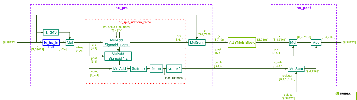
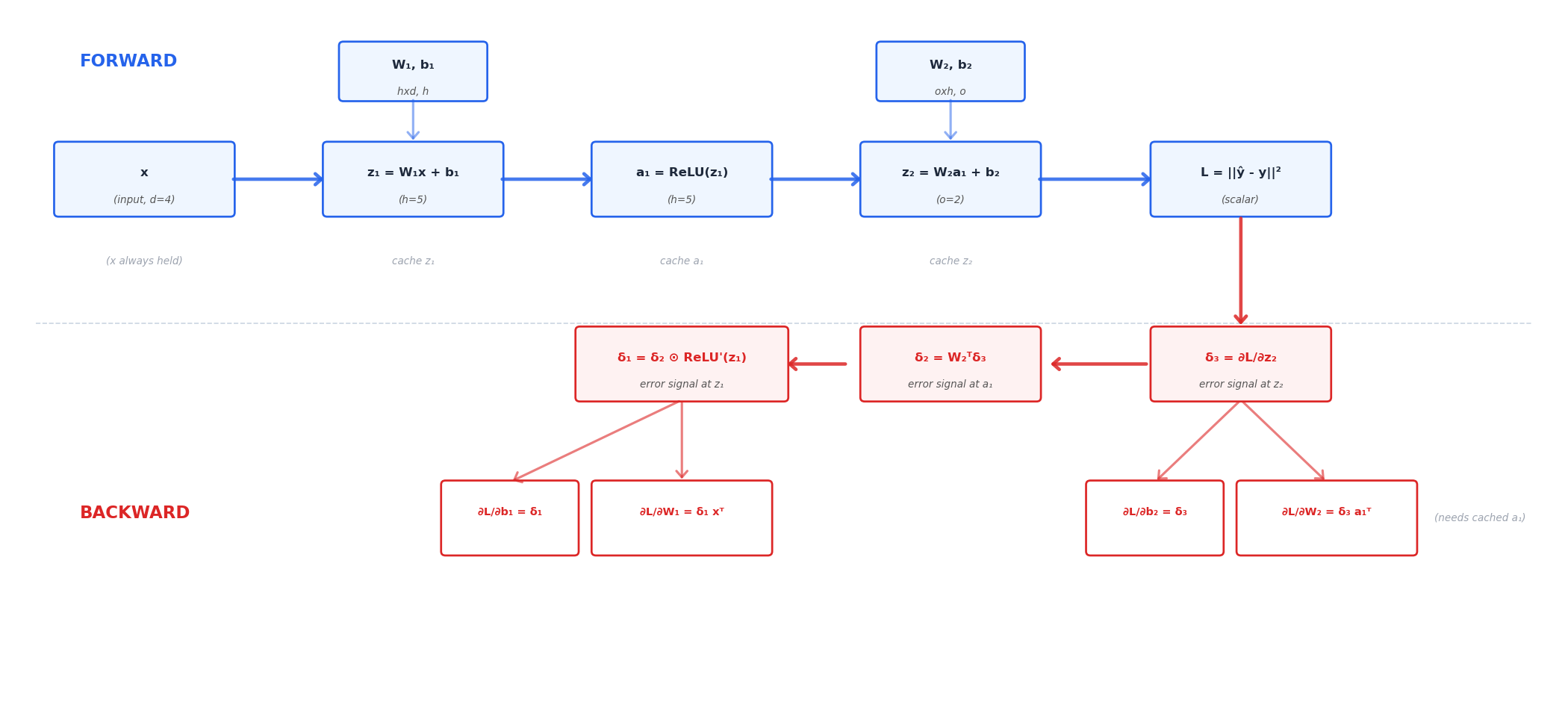
<img src="/assets/images/inference/hc_diagram.png" alt="diagram" /></p>

<p><strong>Figure 1 — mHC dataflow diagram</strong></p>

<p>this diagram i found on flashinfer’s discussion forum is a useful visual reference for understanding the data flow and operations in the mHC preprocessing.</p>

<p><strong>disclaimer:</strong> Claude Opus 4.8 was used to assist my research, as I am not an expert in GPU programming. However this document is 100% my own work and I have done my best to understand the GPU kernels and optimizations used in FlashInfer’s DeepSeek V4.</p>

<h2 id="mhc_pre_big_fusecu">mhc_pre_big_fuse.cu</h2>

<p>I will be going through my understanding of the <a href="https://github.com/flashinfer-ai/flashinfer/pull/3285">mhc_pre_big_fuse kernel</a>. this is an implementation that was merged to flashinfer very recently. I will then explain the optimizations that were made to this kernel and how they improve performance.</p>

<h3 id="the-math-operation">the math operation</h3>
<p>please reference my math document for a better understanding on <strong>why</strong> these operations are needed, and what mHC (manifold-constrained hyper connection) is.
it is available <a href="../2026-06-21-mhc-theory">here</a></p>

<p>for now, I will be assuming you have already went through that resource. Here is how the variables in the math document map to the variables in the kernel code:</p>

<p><strong>Table 1 — Variable map</strong></p>

<table>
  <thead>
    <tr>
      <th>Math Definition</th>
      <th>Kernel Variable</th>
      <th>Data Type</th>
      <th>Dimensions</th>
      <th>Description</th>
    </tr>
  </thead>
  <tbody>
    <tr>
      <td>$X_l$</td>
      <td><code class="language-plaintext highlighter-rouge">residual</code></td>
      <td><code class="language-plaintext highlighter-rouge">__nv_bfloat16</code></td>
      <td>$n_{hc} \times d$</td>
      <td>The input tensor.</td>
    </tr>
    <tr>
      <td>$X_l W_l^{\mathrm{fused}}$</td>
      <td><code class="language-plaintext highlighter-rouge">dot_mix</code></td>
      <td><code class="language-plaintext highlighter-rouge">float</code></td>
      <td>$1 \times (n_{hc} + n_{hc}^2 + n_{hc})$</td>
      <td>The raw output of the fused GEMM projection (calculated before this kernel launches).</td>
    </tr>
    <tr>
      <td>$A_l = \sigma(\tilde A_l) + \epsilon$</td>
      <td><code class="language-plaintext highlighter-rouge">pre_mix</code></td>
      <td><code class="language-plaintext highlighter-rouge">float</code></td>
      <td>$1 \times n_{hc}$</td>
      <td>The compression vector.</td>
    </tr>
    <tr>
      <td>$C_l = 2\cdot\sigma(\tilde C_l)$</td>
      <td><code class="language-plaintext highlighter-rouge">post_mix</code></td>
      <td><code class="language-plaintext highlighter-rouge">float</code></td>
      <td>$n_{hc} \times 1$</td>
      <td>The expansion vector.</td>
    </tr>
    <tr>
      <td>$B_l = \operatorname{Sinkhorn}(\tilde B_l)$</td>
      <td><code class="language-plaintext highlighter-rouge">comb_mix</code></td>
      <td><code class="language-plaintext highlighter-rouge">float</code></td>
      <td>$n_{hc} \times n_{hc}$</td>
      <td>The doubly-stochastic routing matrix.</td>
    </tr>
    <tr>
      <td>$A_l X_l$</td>
      <td><code class="language-plaintext highlighter-rouge">layer_input</code></td>
      <td><code class="language-plaintext highlighter-rouge">__nv_bfloat16</code></td>
      <td>$1 \times d$</td>
      <td>The compressed tensor sent to the MoE/Attention block.</td>
    </tr>
    <tr>
      <td>$\alpha_l^{\text{pre}},\ \alpha_l^{\text{post}},\ \alpha_l^{\text{comb}}$</td>
      <td><code class="language-plaintext highlighter-rouge">mhc_scale[0...2]</code></td>
      <td><code class="language-plaintext highlighter-rouge">float</code></td>
      <td>$3$ (scalars)</td>
      <td>The learnable scalar multipliers for the dynamic components.</td>
    </tr>
    <tr>
      <td>$S_l^{\text{pre}},\ S_l^{\text{post}},\ S_l^{\text{comb}}$</td>
      <td><code class="language-plaintext highlighter-rouge">mhc_base[...]</code></td>
      <td><code class="language-plaintext highlighter-rouge">float</code></td>
      <td>$1 \times (n_{hc} + n_{hc}^2 + n_{hc})$</td>
      <td>The static component offsets.</td>
    </tr>
    <tr>
      <td>$\operatorname{RMS}(X_l)^{-1}$</td>
      <td><code class="language-plaintext highlighter-rouge">rstd</code></td>
      <td><code class="language-plaintext highlighter-rouge">float</code></td>
      <td>$1$ (scalar)</td>
      <td>The reciprocal standard deviation used to finalize the RMSNorm.</td>
    </tr>
  </tbody>
</table>

<p>refresher on $W_l^{\mathrm{fused}}$:</p>

<p>this is a weight matrix, made by concatonating the three weight matrices $W_l^{\text{pre}}, W_l^{\text{post}}, W_l^{\text{comb}}$ along the first dimension. Instead of computing three separate GEMM operations, we can compute one fused GEMM operation to get the same result. This is a common optimization technique in deep learning.</p>

<p>this is included in the math document, but I thought I’d give a refresher.</p>

<h3 id="template-parameters">template parameters:</h3>
<div class="language-cpp highlighter-rouge"><div class="highlight"><pre class="highlight"><code><span class="k">template</span> <span class="o">&lt;</span><span class="kt">int</span> <span class="n">NUM_SPLITS</span><span class="p">,</span> <span class="kt">int</span> <span class="n">BLOCK_SIZE</span><span class="p">,</span> <span class="kt">bool</span> <span class="n">COMPUTE_SQRSUM</span><span class="p">&gt;</span>
</code></pre></div></div>
<p>passing these as template parameters, allows them to be locked at compile time, and the compiler can unroll loops and hardwire memory offsets.</p>

<h3 id="launch-bounds">launch bounds:</h3>

<div class="language-cpp highlighter-rouge"><div class="highlight"><pre class="highlight"><code><span class="n">__launch_bounds__</span><span class="p">(</span><span class="n">BLOCK_SIZE</span><span class="p">)</span>
</code></pre></div></div>
<p>this is an upper bound on the number of threads per block that will be launched for this kernel. the compiler can aggressively optimize for this number of threads instead of being conservative.</p>

<h3 id="function-declaration">function declaration:</h3>
<div class="language-cpp highlighter-rouge"><div class="highlight"><pre class="highlight"><code><span class="n">__global__</span> <span class="kt">void</span> <span class="n">mhc_pre_big_fuse_kernel</span><span class="p">(...)</span>
</code></pre></div></div>

<p>standard cuda kernel declaration. the variables were already explained in the table above.</p>

<h4 id="special-flags-used">special flags used:</h4>
<div class="language-cpp highlighter-rouge"><div class="highlight"><pre class="highlight"><code><span class="k">const</span> <span class="kt">float</span><span class="o">*</span> <span class="n">__restrict__</span> <span class="n">dot_mix</span><span class="p">,</span> 
<span class="k">const</span> <span class="n">__nv_bfloat16</span><span class="o">*</span> <span class="n">__restrict__</span> <span class="n">residual</span><span class="p">,</span>
</code></pre></div></div>
<p>restrict promises the compiler that these pointers are not aliased. meaning, they’ll never point at the same memory. Without this, the compiler won’t pull data from these addresses to read only caches for optimization.</p>

<h3 id="hardware-data-types">hardware data types:</h3>
<div class="language-cpp highlighter-rouge"><div class="highlight"><pre class="highlight"><code><span class="n">__nv_bfloat16</span><span class="p">,</span> <span class="kt">float</span>
</code></pre></div></div>

<p><strong>Table 2 — Hardware data types</strong></p>

<table>
  <thead>
    <tr>
      <th style="text-align: right">Type</th>
      <th style="text-align: center">Bits</th>
      <th style="text-align: center">Exponent</th>
      <th style="text-align: center">Mantissa</th>
      <th style="text-align: left">Approx. Range</th>
      <th>Notes</th>
    </tr>
  </thead>
  <tbody>
    <tr>
      <td style="text-align: right"><code class="language-plaintext highlighter-rouge">fp32</code> (IEEE-754)</td>
      <td style="text-align: center">32</td>
      <td style="text-align: center">8</td>
      <td style="text-align: center">23</td>
      <td style="text-align: left">~1e±38</td>
      <td>Single precision; standard for training and many kernels.</td>
    </tr>
    <tr>
      <td style="text-align: right"><code class="language-plaintext highlighter-rouge">fp16</code> (IEEE-754 half)</td>
      <td style="text-align: center">16</td>
      <td style="text-align: center">5</td>
      <td style="text-align: center">10</td>
      <td style="text-align: left">max ≈ 6.55e4</td>
      <td>Lower precision and range; accelerated on Tensor Cores (fast but reduced numeric fidelity).</td>
    </tr>
    <tr>
      <td style="text-align: right"><code class="language-plaintext highlighter-rouge">bfloat16</code></td>
      <td style="text-align: center">16</td>
      <td style="text-align: center">8</td>
      <td style="text-align: center">7</td>
      <td style="text-align: left">~1e±38</td>
      <td>Same exponent as <code class="language-plaintext highlighter-rouge">fp32</code> (large dynamic range) with reduced precision — often helps training stability.</td>
    </tr>
    <tr>
      <td style="text-align: right"><code class="language-plaintext highlighter-rouge">__nv_bfloat16</code></td>
      <td style="text-align: center">16</td>
      <td style="text-align: center">8</td>
      <td style="text-align: center">7</td>
      <td style="text-align: left">~1e±38</td>
      <td>NVIDIA CUDA bfloat16 type; hardware-accelerated on many modern NVIDIA GPUs (data-center architectures).</td>
    </tr>
  </tbody>
</table>

<p>as documented in Table 1, params like the mix vectors, and rstd are kept in high precision, as they are used in operations that require full numerical accuracy.
but where possible ((for example the residual itself), we use the lower-precision <code class="language-plaintext highlighter-rouge">__nv_bfloat16</code> type to save memory bandwidth and storage, while still maintaining a large dynamic range.</p>

<h3 id="static-asserts">static asserts</h3>

<div class="language-cpp highlighter-rouge"><div class="highlight"><pre class="highlight"><code><span class="k">static_assert</span><span class="p">(</span><span class="n">NUM_SPLITS</span> <span class="o">==</span> <span class="mi">1</span> <span class="o">||</span> <span class="o">!</span><span class="n">COMPUTE_SQRSUM</span><span class="p">,</span>
              <span class="s">"internal sqrsum path only supports NUM_SPLITS=1"</span><span class="p">);</span>
</code></pre></div></div>
<p>static_assert acts as a fail-safe. It stops the code from even compiling if someone tries to launch the kernel with an unsupported combination of optimizations.</p>

<h3 id="high-level-overview-of-the-kernel-and-the-optimizations-applied">high level overview of the kernel and the optimizations applied</h3>
<h4 id="one-token--one-block">one token = one block</h4>
<p>each thread block is responsible for processing one token.</p>

<p>this makes things simpler, because my math document (and the deepseek paper) both describe the mHC operations on a per-token basis. so we can directly map the math to the code without worrying about how multiple tokens are handled within a block.</p>

<h4 id="warp-0-vs-warps-1">warp 0 vs warps 1+</h4>

<p>the kernel is designed such that warp 0 (specifically the first 4 threads in the block) is responsible for computing the metadata (the mix vectors and the routing matrix), while warps 1+ are responsible for the reduction to compute the final output.</p>

<div class="language-cpp highlighter-rouge"><div class="highlight"><pre class="highlight"><code><span class="k">const</span> <span class="kt">int</span> <span class="n">warp_id</span> <span class="o">=</span> <span class="n">threadIdx</span><span class="p">.</span><span class="n">x</span> <span class="o">/</span> <span class="n">kWarpThreads</span><span class="p">;</span>
<span class="k">const</span> <span class="kt">int</span> <span class="n">lane</span> <span class="o">=</span> <span class="n">threadIdx</span><span class="p">.</span><span class="n">x</span> <span class="o">&amp;</span> <span class="p">(</span><span class="n">kWarpThreads</span> <span class="o">-</span> <span class="mi">1</span><span class="p">);</span>
<span class="k">const</span> <span class="kt">bool</span> <span class="n">meta_lane</span> <span class="o">=</span> <span class="p">(</span><span class="n">warp_id</span> <span class="o">==</span> <span class="mi">0</span> <span class="o">&amp;&amp;</span> <span class="n">lane</span> <span class="o">&lt;</span> <span class="n">kHc4</span><span class="p">);</span>
</code></pre></div></div>

<p><code class="language-plaintext highlighter-rouge">kHc4 = 4</code>, meaning this kernel is specialized for exactly 4 hyper-connection lanes.</p>

<h3 id="constants-in-the-kernel">constants in the kernel</h3>

<p>at the top of the file we have:</p>

<div class="language-cpp highlighter-rouge"><div class="highlight"><pre class="highlight"><code><span class="k">static</span> <span class="k">constexpr</span> <span class="kt">int</span> <span class="n">kHc4</span> <span class="o">=</span> <span class="mi">4</span><span class="p">;</span>
<span class="k">static</span> <span class="k">constexpr</span> <span class="kt">int</span> <span class="n">kMixHc4</span> <span class="o">=</span> <span class="n">kHc4</span> <span class="o">*</span> <span class="p">(</span><span class="mi">2</span> <span class="o">+</span> <span class="n">kHc4</span><span class="p">);</span>
<span class="k">static</span> <span class="k">constexpr</span> <span class="kt">int</span> <span class="n">kWarpThreads</span> <span class="o">=</span> <span class="mi">32</span><span class="p">;</span>
<span class="k">static</span> <span class="k">constexpr</span> <span class="kt">int</span> <span class="n">kVecWidth</span> <span class="o">=</span> <span class="mi">8</span><span class="p">;</span>
</code></pre></div></div>

<p>these constants tell us a lot about how the kernel is designed.</p>

<p><strong>Table 3 — Kernel constants</strong></p>

<table>
  <thead>
    <tr>
      <th>Constant</th>
      <th>Value</th>
      <th style="text-align: right">Meaning</th>
    </tr>
  </thead>
  <tbody>
    <tr>
      <td><code class="language-plaintext highlighter-rouge">kHc4</code></td>
      <td>4</td>
      <td style="text-align: right">number of hyper-connection lanes.</td>
    </tr>
    <tr>
      <td><code class="language-plaintext highlighter-rouge">kMixHc4</code></td>
      <td>24</td>
      <td style="text-align: right">total metadata values per token: 4 pre + 4 post + 16 comb.</td>
    </tr>
    <tr>
      <td><code class="language-plaintext highlighter-rouge">kWarpThreads</code></td>
      <td>32</td>
      <td style="text-align: right">CUDA warp size.</td>
    </tr>
    <tr>
      <td><code class="language-plaintext highlighter-rouge">kVecWidth</code></td>
      <td>8</td>
      <td style="text-align: right">each vectorized load/store handles 8 bf16 values.</td>
    </tr>
  </tbody>
</table>

<p>why <code class="language-plaintext highlighter-rouge">kMixHc4 = 24</code>?</p>

\[4 + 4 + 4^2 = 24\]

<p>this is exactly:</p>

\[A_l \text{ params} + C_l \text{ params} + B_l \text{ params}\]

<p>so for every token, <code class="language-plaintext highlighter-rouge">dot_mix</code> stores 24 float values generated by the previous fused GEMM.</p>

<h3 id="vectorized-bf16-loads-and-stores">vectorized bf16 loads and stores</h3>

<p>the kernel defines a small helper struct:</p>

<div class="language-cpp highlighter-rouge"><div class="highlight"><pre class="highlight"><code><span class="k">struct</span> <span class="nc">Bf16x8</span> <span class="p">{</span>
  <span class="n">uint4</span> <span class="n">raw</span><span class="p">;</span>
<span class="p">};</span>
</code></pre></div></div>

<p><code class="language-plaintext highlighter-rouge">uint4</code> is 4 unsigned 32-bit values, so total size is:</p>

\[4 \times 32 = 128 \text{ bits} = 16 \text{ bytes}\]

<p>since bf16 is 16 bits, 16 bytes contains:</p>

\[16 \text{ bytes} / 2 \text{ bytes per bf16} = 8 \text{ bf16 values}\]

<p>this is why it is called <code class="language-plaintext highlighter-rouge">Bf16x8</code>.</p>

<div class="language-cpp highlighter-rouge"><div class="highlight"><pre class="highlight"><code><span class="k">asm</span> <span class="k">volatile</span><span class="p">(</span><span class="s">"ld.global.v4.u32 {%0, %1, %2, %3}, [%4];</span><span class="se">\n</span><span class="s">"</span> <span class="p">...)</span>
<span class="k">asm</span> <span class="k">volatile</span><span class="p">(</span><span class="s">"st.global.v4.u32 [%4], {%0, %1, %2, %3};</span><span class="se">\n</span><span class="s">"</span> <span class="p">...)</span>
</code></pre></div></div>

<p>Here, we use inline PTX assembly. We force the compiler to load 128-bits of data (in the form of a vector of 8 bf16 values)from the global memory, utilizing the whole bus. this is known as “manual emission”.</p>

<h3 id="square-sum-and-rmsnorm">square sum and RMSNorm</h3>

<p>there are two ways the kernel can get the RMSNorm denominator.</p>

<h4 id="path-1-sqrsum-is-already-provided">path 1: sqrsum is already provided</h4>

<p>in the normal <code class="language-plaintext highlighter-rouge">mhc_pre_big_fuse</code> function, <code class="language-plaintext highlighter-rouge">sqrsum</code> is passed in from outside:</p>

<div class="language-cpp highlighter-rouge"><div class="highlight"><pre class="highlight"><code><span class="k">const</span> <span class="kt">float</span><span class="o">*</span> <span class="n">__restrict__</span> <span class="n">sqrsum</span>
</code></pre></div></div>

<p>if <code class="language-plaintext highlighter-rouge">COMPUTE_SQRSUM == false</code>, then the kernel does:</p>

<div class="language-cpp highlighter-rouge"><div class="highlight"><pre class="highlight"><code><span class="n">sq_total</span> <span class="o">=</span> <span class="n">sqrsum</span><span class="p">[</span><span class="n">token</span><span class="p">];</span>
</code></pre></div></div>

<p>or if split-K was used:</p>

<div class="language-cpp highlighter-rouge"><div class="highlight"><pre class="highlight"><code><span class="n">sq_total</span> <span class="o">+=</span> <span class="n">sqrsum</span><span class="p">[</span><span class="n">s</span> <span class="o">*</span> <span class="n">total_tokens</span> <span class="o">+</span> <span class="n">token</span><span class="p">];</span>
</code></pre></div></div>

<p>so the square sum was computed before this kernel, probably during the previous projection/reduction stage.</p>

<h4 id="path-2-compute-sqrsum-inside-this-kernel">path 2: compute sqrsum inside this kernel</h4>

<p>there is also a <code class="language-plaintext highlighter-rouge">mhc_pre_big_fuse_with_prenorm</code> function. In that path, the kernel launches with:</p>

<div class="language-cpp highlighter-rouge"><div class="highlight"><pre class="highlight"><code><span class="n">dispatch_pre_big_fuse</span><span class="o">&lt;</span><span class="mi">1</span><span class="p">,</span> <span class="nb">true</span><span class="o">&gt;</span><span class="p">(...)</span>
</code></pre></div></div>

<p>so <code class="language-plaintext highlighter-rouge">COMPUTE_SQRSUM = true</code>.</p>

<p>then the kernel runs:</p>

<div class="language-cpp highlighter-rouge"><div class="highlight"><pre class="highlight"><code><span class="k">const</span> <span class="kt">float</span> <span class="n">local_sq</span> <span class="o">=</span> <span class="n">residual_square_sum_vec8</span><span class="o">&lt;</span><span class="n">BLOCK_SIZE</span><span class="o">&gt;</span><span class="p">(</span><span class="n">residual_token</span><span class="p">,</span> <span class="n">kHc4</span> <span class="o">*</span> <span class="n">H</span><span class="p">);</span>
<span class="n">sq_total</span> <span class="o">=</span> <span class="n">block_sum</span><span class="o">&lt;</span><span class="n">BLOCK_SIZE</span><span class="o">&gt;</span><span class="p">(</span><span class="n">local_sq</span><span class="p">,</span> <span class="n">sq_partials</span><span class="p">);</span>
</code></pre></div></div>

<p>this streams through the residual tensor, squares every element, and reduces it inside the block. “reducing” here means taking the sum across the feature dimension, so we end up with the total sum of squares for that token. This is callde a “reduction” operation in parallel programming, because we are reducing a large set of values down to a single value (the total sum).</p>

<p>mathematically this is computing:</p>

\[\sum_i X_i^2\]

<p>then the reciprocal RMS is:</p>

<div class="language-cpp highlighter-rouge"><div class="highlight"><pre class="highlight"><code><span class="n">rstd</span> <span class="o">=</span> <span class="n">rsqrtf</span><span class="p">(</span><span class="n">sq_total</span> <span class="o">/</span> <span class="k">static_cast</span><span class="o">&lt;</span><span class="kt">float</span><span class="o">&gt;</span><span class="p">(</span><span class="n">K</span><span class="p">)</span> <span class="o">+</span> <span class="n">rms_eps</span><span class="p">);</span>
</code></pre></div></div>

<p>which maps to:</p>

\[rstd = \frac{1}{\sqrt{\frac{1}{K}\sum_i X_i^2 + \epsilon}}\]

<p>this is exactly the denominator of RMSNorm.</p>

<h3 id="block-reduction-details">block reduction details</h3>

<p>there are two reduction helpers:</p>

<div class="language-cpp highlighter-rouge"><div class="highlight"><pre class="highlight"><code><span class="n">warp_sum</span><span class="p">(</span><span class="kt">float</span> <span class="n">v</span><span class="p">)</span>
<span class="n">block_sum</span><span class="o">&lt;</span><span class="n">BLOCK_SIZE</span><span class="o">&gt;</span><span class="p">(</span><span class="kt">float</span> <span class="n">v</span><span class="p">,</span> <span class="kt">float</span><span class="o">*</span> <span class="n">shared</span><span class="p">)</span>
</code></pre></div></div>

<p><code class="language-plaintext highlighter-rouge">warp_sum</code> uses warp shuffle instructions:</p>

<div class="language-cpp highlighter-rouge"><div class="highlight"><pre class="highlight"><code><span class="n">v</span> <span class="o">+=</span> <span class="n">__shfl_down_sync</span><span class="p">(</span><span class="mh">0xffffffffu</span><span class="p">,</span> <span class="n">v</span><span class="p">,</span> <span class="n">offset</span><span class="p">);</span>
</code></pre></div></div>

<p>this reduces values inside one warp without shared memory. This is faster than writing every partial sum to shared memory, because warp lanes can exchange register values directly.</p>

<p><code class="language-plaintext highlighter-rouge">block_sum</code> then does a two-stage reduction:</p>

<ol>
  <li>every warp reduces its own lanes using <code class="language-plaintext highlighter-rouge">warp_sum</code></li>
  <li>lane 0 of each warp writes a partial sum to shared memory</li>
  <li>warp 0 reduces those warp-level partial sums</li>
  <li>thread 0 publishes the final result back into shared memory</li>
</ol>

<p>this is a standard fast block reduction pattern.</p>

<h3 id="original-path-vs-my-h100-path">original path vs my h100 path</h3>

<p>there are two versions of the metadata generation in the same kernel. The first one is the original/general implementation, and the second one is the H100-specific path I added after looking through the generated code and profiling behavior.</p>

<div class="language-cpp highlighter-rouge"><div class="highlight"><pre class="highlight"><code><span class="cp">#if defined(__CUDA_ARCH__) &amp;&amp; (__CUDA_ARCH__ == 900)
</span>  <span class="c1">// Hopper fast path</span>
<span class="cp">#else
</span>  <span class="c1">// Portable path</span>
<span class="cp">#endif
</span></code></pre></div></div>

<p><code class="language-plaintext highlighter-rouge">__CUDA_ARCH__ == 900</code> means the code is being compiled for sm90, which is H100/Hopper. This lets us keep the original path available for other architectures, while specializing the hot path for the hardware I was targeting.</p>

<h4 id="the-originalgeneral-path">the original/general path</h4>

<p>the original code took a general path, with decent portability and readable structure. here, warp 0 uses a local array:</p>

<div class="language-cpp highlighter-rouge"><div class="highlight"><pre class="highlight"><code><span class="kt">float</span> <span class="n">y_local</span><span class="p">[</span><span class="n">kMixHc4</span><span class="p">];</span>
</code></pre></div></div>

<p>that is 24 floats.</p>

\[24 \times 4 \text{ bytes} = 96 \text{ bytes}\]

<p>then it loads the full metadata row:</p>

<div class="language-cpp highlighter-rouge"><div class="highlight"><pre class="highlight"><code><span class="k">for</span> <span class="p">(</span><span class="kt">int</span> <span class="n">c</span> <span class="o">=</span> <span class="mi">0</span><span class="p">;</span> <span class="n">c</span> <span class="o">&lt;</span> <span class="n">kMixHc4</span><span class="p">;</span> <span class="o">++</span><span class="n">c</span><span class="p">)</span> <span class="p">{</span>
  <span class="n">y_local</span><span class="p">[</span><span class="n">c</span><span class="p">]</span> <span class="o">=</span> <span class="n">y_row</span><span class="p">[</span><span class="n">c</span><span class="p">];</span>
<span class="p">}</span>
</code></pre></div></div>

<p>and calls:</p>

<div class="language-cpp highlighter-rouge"><div class="highlight"><pre class="highlight"><code><span class="n">write_token_metadata</span><span class="p">(</span><span class="n">y_local</span><span class="p">,</span> <span class="n">rstd</span><span class="p">,</span> <span class="p">...)</span>
</code></pre></div></div>

<p>this code is clean, and it matches the math nicely. But the issue I found is that the helper function uses lane-dependent indexing:</p>

<div class="language-cpp highlighter-rouge"><div class="highlight"><pre class="highlight"><code><span class="n">y_local</span><span class="p">[</span><span class="n">lane</span><span class="p">]</span>
<span class="n">y_local</span><span class="p">[</span><span class="n">kHc4</span> <span class="o">+</span> <span class="n">lane</span><span class="p">]</span>
<span class="n">y_local</span><span class="p">[</span><span class="mi">2</span> <span class="o">*</span> <span class="n">kHc4</span> <span class="o">+</span> <span class="n">lane</span> <span class="o">*</span> <span class="n">kHc4</span> <span class="o">+</span> <span class="n">k</span><span class="p">]</span>
</code></pre></div></div>

<p>from the programmer’s perspective this is obvious: lane 0 handles row 0, lane 1 handles row 1, etc.</p>

<p>but from the compiler’s perspective, <code class="language-plaintext highlighter-rouge">lane</code> is dynamic. It is not a compile-time constant. The compiler may not be able to keep the whole <code class="language-plaintext highlighter-rouge">y_local</code> array in registers, because indexing into an array with a dynamic index often forces it to put that array into local memory.</p>

<p>Note: CUDA “local memory” is not the same as a CPU local variable. It usually spills to global memory and is cached. So if <code class="language-plaintext highlighter-rouge">y_local</code> spills, the metadata warp now has extra global-memory traffic just to access 96 bytes of temporary values.</p>

<p>this was in fact occouring when I inspected the <code class="language-plaintext highlighter-rouge">cuobjdump</code> output <code class="language-plaintext highlighter-rouge">STACK:96</code>. I could see the register spill/local-memory behavior there, even though I could not dynamically inspect it with Nsight on an H100. That was the first clue that the nice modular helper function was costing us real performance.</p>

<p>I verified after the fix and <code class="language-plaintext highlighter-rouge">STACK:0, LOCAL:0</code> there was no local memory spill, and the kernel was now fully register-resident for the metadata work.</p>

<p>The second clue was the warp scheduling. Warps 1+ were blocked at the barrier while warp 0 finished all the metadata work, including the Sinkhorn loop. So the kernel had two problems:</p>

<ol>
  <li>warp 0 was slower than it needed to be because of the local-memory spill.</li>
  <li>the rest of the block was waiting for warp 0, even though it only needed <code class="language-plaintext highlighter-rouge">pre_mix</code>.</li>
</ol>

<p>I used claude to confirm these observations, and breakdown how to fix the issue.</p>

<h4 id="my-h100-path">my h100 path</h4>

<p>on H100, I changed the path to avoid the <code class="language-plaintext highlighter-rouge">y_local[24]</code> temporary and instead keep only what each lane actually needs.</p>

<p>for each metadata lane:</p>

<div class="language-cpp highlighter-rouge"><div class="highlight"><pre class="highlight"><code><span class="kt">float</span> <span class="n">y_pre</span> <span class="o">=</span> <span class="mf">0.0</span><span class="n">f</span><span class="p">;</span>
<span class="kt">float</span> <span class="n">y_post</span> <span class="o">=</span> <span class="mf">0.0</span><span class="n">f</span><span class="p">;</span>
<span class="kt">float</span> <span class="n">cmv</span><span class="p">[</span><span class="n">kHc4</span><span class="p">];</span>
</code></pre></div></div>

<p>so lane 0 only holds the row needed for lane 0, lane 1 holds the row needed for lane 1, and so on.</p>

<p>for <code class="language-plaintext highlighter-rouge">NUM_SPLITS == 1</code>, the load is:</p>

<div class="language-cpp highlighter-rouge"><div class="highlight"><pre class="highlight"><code><span class="n">y_pre</span> <span class="o">=</span> <span class="n">y_row</span><span class="p">[</span><span class="n">lane</span><span class="p">];</span>
<span class="n">y_post</span> <span class="o">=</span> <span class="n">y_row</span><span class="p">[</span><span class="n">kHc4</span> <span class="o">+</span> <span class="n">lane</span><span class="p">];</span>
<span class="k">for</span> <span class="p">(</span><span class="kt">int</span> <span class="n">k</span> <span class="o">=</span> <span class="mi">0</span><span class="p">;</span> <span class="n">k</span> <span class="o">&lt;</span> <span class="n">kHc4</span><span class="p">;</span> <span class="o">++</span><span class="n">k</span><span class="p">)</span> <span class="p">{</span>
  <span class="n">cmv</span><span class="p">[</span><span class="n">k</span><span class="p">]</span> <span class="o">=</span> <span class="n">y_row</span><span class="p">[</span><span class="mi">2</span> <span class="o">*</span> <span class="n">kHc4</span> <span class="o">+</span> <span class="n">lane</span> <span class="o">*</span> <span class="n">kHc4</span> <span class="o">+</span> <span class="n">k</span><span class="p">];</span>
<span class="p">}</span>
</code></pre></div></div>

<p>this is much more register friendly. <code class="language-plaintext highlighter-rouge">cmv[k]</code> is accessed with unrolled constant <code class="language-plaintext highlighter-rouge">k</code>, and there is no 24-element array indexed by a dynamic lane id. The goal was very direct: keep the metadata slice in registers and stop paying local-memory traffic for a tiny 96-byte temporary.</p>

<p>for split-K, it accumulates the same slice across splits:</p>

<div class="language-cpp highlighter-rouge"><div class="highlight"><pre class="highlight"><code><span class="k">for</span> <span class="p">(</span><span class="kt">int</span> <span class="n">s</span> <span class="o">=</span> <span class="mi">0</span><span class="p">;</span> <span class="n">s</span> <span class="o">&lt;</span> <span class="n">NUM_SPLITS</span><span class="p">;</span> <span class="o">++</span><span class="n">s</span><span class="p">)</span> <span class="p">{</span>
  <span class="n">sq_total</span> <span class="o">+=</span> <span class="n">sqrsum</span><span class="p">[</span><span class="n">s</span> <span class="o">*</span> <span class="n">total_tokens</span> <span class="o">+</span> <span class="n">token</span><span class="p">];</span>
  <span class="k">const</span> <span class="kt">float</span><span class="o">*</span> <span class="n">y_row</span> <span class="o">=</span> <span class="n">dot_mix</span> <span class="o">+</span> <span class="p">(</span><span class="n">s</span> <span class="o">*</span> <span class="n">total_tokens</span> <span class="o">+</span> <span class="n">token</span><span class="p">)</span> <span class="o">*</span> <span class="n">kMixHc4</span><span class="p">;</span>
  <span class="n">y_pre</span> <span class="o">+=</span> <span class="n">y_row</span><span class="p">[</span><span class="n">lane</span><span class="p">];</span>
  <span class="n">y_post</span> <span class="o">+=</span> <span class="n">y_row</span><span class="p">[</span><span class="n">kHc4</span> <span class="o">+</span> <span class="n">lane</span><span class="p">];</span>
  <span class="k">for</span> <span class="p">(</span><span class="kt">int</span> <span class="n">k</span> <span class="o">=</span> <span class="mi">0</span><span class="p">;</span> <span class="n">k</span> <span class="o">&lt;</span> <span class="n">kHc4</span><span class="p">;</span> <span class="o">++</span><span class="n">k</span><span class="p">)</span> <span class="p">{</span>
    <span class="n">cmv</span><span class="p">[</span><span class="n">k</span><span class="p">]</span> <span class="o">+=</span> <span class="n">y_row</span><span class="p">[</span><span class="mi">2</span> <span class="o">*</span> <span class="n">kHc4</span> <span class="o">+</span> <span class="n">lane</span> <span class="o">*</span> <span class="n">kHc4</span> <span class="o">+</span> <span class="n">k</span><span class="p">];</span>
  <span class="p">}</span>
<span class="p">}</span>
</code></pre></div></div>

<p>this is the same idea for split-K. each split produces a partial <code class="language-plaintext highlighter-rouge">dot_mix</code>, and this path accumulates only the values this lane owns instead of rebuilding the full 24-float row.</p>

<h3 id="explaining-split-k">explaining split-K</h3>

<p>for one token, the fused projection is:</p>

\[\hat{X_l} W_l^{fused}\]

<p>but $\hat{X_l}$ is huge because it is the flattened 4-lane residual:</p>

\[\hat{X_l} \in R^{1 \times (4d)}\]

<p>and for DeepSeek-style hidden sizes, $d$ can be very large.</p>

<p>Split-K means the previous GEMM can split the long K dimension into chunks. Each chunk computes a partial dot product, and then this kernel adds those partial dot products:</p>

\[dot\_mix = \sum_s dot\_mix^{(s)}\]

<p>same for the square sum:</p>

\[sqrsum = \sum_s sqrsum^{(s)}\]

<p>why this helps: if the GEMM is too skinny or has too few output columns (only 24 values per token), split-K can create more parallel work for the GPU. It trades an extra reduction for better occupancy/utilization in the projection stage.</p>

<h3 id="computing-pre_mix-early">computing pre_mix early</h3>

<p>this was the second optimization I made. After fixing the register/local-memory issue, the next obvious waste was that most of the block was just sitting at the barrier.</p>

<p>The old logical order was:</p>

<ol>
  <li>load all metadata</li>
  <li>compute <code class="language-plaintext highlighter-rouge">pre_mix</code></li>
  <li>compute <code class="language-plaintext highlighter-rouge">post_mix</code></li>
  <li>run Sinkhorn for <code class="language-plaintext highlighter-rouge">comb_mix</code></li>
  <li><code class="language-plaintext highlighter-rouge">__syncthreads()</code></li>
  <li>compute <code class="language-plaintext highlighter-rouge">layer_input = A_l X_l</code></li>
</ol>

<p>that is easy to read, but bad for overlap. Warps 1+ are idle while warp 0 does all the scalar metadata math.</p>

<p>The thing I noticed is that warps 1+ do not need all metadata. They only need <code class="language-plaintext highlighter-rouge">pre_mix</code>, because their job is just:</p>

\[layer\_input = A_l X_l\]

<p>so I changed the order:</p>

<ol>
  <li>warp 0 loads metadata slice</li>
  <li>warp 0 computes only <code class="language-plaintext highlighter-rouge">pre_mix</code></li>
  <li><code class="language-plaintext highlighter-rouge">__syncthreads()</code> publishes <code class="language-plaintext highlighter-rouge">pre_mix</code></li>
  <li>warps 1+ start computing <code class="language-plaintext highlighter-rouge">layer_input</code></li>
  <li>meanwhile, warp 0 computes <code class="language-plaintext highlighter-rouge">post_mix</code> and <code class="language-plaintext highlighter-rouge">comb_mix</code></li>
</ol>

<p>the code now reflects that split:</p>

<div class="language-cpp highlighter-rouge"><div class="highlight"><pre class="highlight"><code><span class="k">if</span> <span class="p">(</span><span class="n">meta_lane</span><span class="p">)</span> <span class="p">{</span>
  <span class="p">...</span>
  <span class="n">rstd</span> <span class="o">=</span> <span class="n">rsqrtf</span><span class="p">(...);</span>
  <span class="k">const</span> <span class="kt">float</span> <span class="n">v</span> <span class="o">=</span> <span class="n">y_pre</span> <span class="o">*</span> <span class="n">rstd</span> <span class="o">*</span> <span class="n">mhc_scale</span><span class="p">[</span><span class="mi">0</span><span class="p">]</span> <span class="o">+</span> <span class="n">mhc_base</span><span class="p">[</span><span class="n">lane</span><span class="p">];</span>
  <span class="n">pre_mix</span><span class="p">[</span><span class="n">lane</span><span class="p">]</span> <span class="o">=</span> <span class="mf">1.0</span><span class="n">f</span> <span class="o">/</span> <span class="p">(</span><span class="mf">1.0</span><span class="n">f</span> <span class="o">+</span> <span class="n">expf</span><span class="p">(</span><span class="o">-</span><span class="n">v</span><span class="p">))</span> <span class="o">+</span> <span class="n">mhc_pre_eps</span><span class="p">;</span>
<span class="p">}</span>

<span class="n">__syncthreads</span><span class="p">();</span>

<span class="k">if</span> <span class="p">(</span><span class="n">meta_lane</span><span class="p">)</span> <span class="p">{</span>
  <span class="c1">// post_mix and Sinkhorn happen here</span>
<span class="p">}</span>

<span class="n">write_layer_input</span><span class="o">&lt;</span><span class="n">BLOCK_SIZE</span><span class="o">&gt;</span><span class="p">(...);</span>
</code></pre></div></div>

<p>after this, the kernel no longer waits for the Sinkhorn loop before starting the heavy memory streaming work.</p>

<p>main idea: move the barrier to the first real dependency. not after all metadata is done, only after <code class="language-plaintext highlighter-rouge">pre_mix</code> is ready.</p>

<h3 id="execution-timeline">execution timeline</h3>

<p>here is the optimized execution flow:</p>

<pre><code class="language-mermaid">flowchart TD
    A[block starts: one token] --&gt; B{COMPUTE_SQRSUM?}
    B --&gt;|yes| C[all threads compute residual square sum]
    B --&gt;|no| D[warp 0 reads sqrsum]
    C --&gt; E[warp 0 lanes 0 to 3 load dot_mix slice]
    D --&gt; E
    E --&gt; F[warp 0 computes rstd and pre_mix]
    F --&gt; G[__syncthreads publishes pre_mix]
    G --&gt; H[warps 1+ compute layer_input = A_l X_l]
    G --&gt; I[warp 0 computes post_mix]
    I --&gt; J[warp 0 runs Sinkhorn]
    J --&gt; K[warp 0 writes comb_mix]
    H --&gt; L[block done]
    K --&gt; L
</code></pre>

<p>this diagram is a bit simplified, but the key idea is that after the barrier, two independent pieces of work happen at the same time:</p>

<ul>
  <li>warp 0 does scalar-heavy metadata work</li>
  <li>warps 1+ do bandwidth-heavy residual compression</li>
</ul>

<h3 id="computing-a_l-pre_mix">computing $A_l$ (pre_mix)</h3>

<p>The pre-mix gate is:</p>

\[A_l = \sigma(\tilde A_l) + \epsilon\]

<p>in code:</p>

<div class="language-cpp highlighter-rouge"><div class="highlight"><pre class="highlight"><code><span class="k">const</span> <span class="kt">float</span> <span class="n">v</span> <span class="o">=</span> <span class="n">y_pre</span> <span class="o">*</span> <span class="n">rstd</span> <span class="o">*</span> <span class="n">mhc_scale</span><span class="p">[</span><span class="mi">0</span><span class="p">]</span> <span class="o">+</span> <span class="n">mhc_base</span><span class="p">[</span><span class="n">lane</span><span class="p">];</span>
<span class="n">pre_mix</span><span class="p">[</span><span class="n">lane</span><span class="p">]</span> <span class="o">=</span> <span class="mf">1.0</span><span class="n">f</span> <span class="o">/</span> <span class="p">(</span><span class="mf">1.0</span><span class="n">f</span> <span class="o">+</span> <span class="n">expf</span><span class="p">(</span><span class="o">-</span><span class="n">v</span><span class="p">))</span> <span class="o">+</span> <span class="n">mhc_pre_eps</span><span class="p">;</span>
</code></pre></div></div>

<p>mapping:</p>

<table>
  <thead>
    <tr>
      <th>Math</th>
      <th>Code</th>
    </tr>
  </thead>
  <tbody>
    <tr>
      <td>dynamic projection output</td>
      <td><code class="language-plaintext highlighter-rouge">y_pre</code></td>
    </tr>
    <tr>
      <td>RMSNorm scaling</td>
      <td><code class="language-plaintext highlighter-rouge">rstd</code></td>
    </tr>
    <tr>
      <td>dynamic scale</td>
      <td><code class="language-plaintext highlighter-rouge">mhc_scale[0]</code></td>
    </tr>
    <tr>
      <td>static base</td>
      <td><code class="language-plaintext highlighter-rouge">mhc_base[lane]</code></td>
    </tr>
    <tr>
      <td>non-zero floor</td>
      <td><code class="language-plaintext highlighter-rouge">mhc_pre_eps</code></td>
    </tr>
  </tbody>
</table>

<p>so:</p>

\[\tilde A_l = y_{pre} \cdot rstd \cdot \alpha_l^{pre} + S_l^{pre}\]

\[A_l = \sigma(\tilde A_l) + \epsilon\]

<h3 id="computing-c_l-post_mix">computing $C_l$ (post_mix)</h3>

<p>After the barrier, warp 0 computes post-mix:</p>

<div class="language-cpp highlighter-rouge"><div class="highlight"><pre class="highlight"><code><span class="k">const</span> <span class="kt">float</span> <span class="n">vp</span> <span class="o">=</span> <span class="n">y_post</span> <span class="o">*</span> <span class="n">rstd</span> <span class="o">*</span> <span class="n">mhc_scale</span><span class="p">[</span><span class="mi">1</span><span class="p">]</span> <span class="o">+</span> <span class="n">mhc_base</span><span class="p">[</span><span class="n">kHc4</span> <span class="o">+</span> <span class="n">lane</span><span class="p">];</span>
<span class="n">post_mix</span><span class="p">[</span><span class="n">token</span> <span class="o">*</span> <span class="n">kHc4</span> <span class="o">+</span> <span class="n">lane</span><span class="p">]</span> <span class="o">=</span>
    <span class="mf">1.0</span><span class="n">f</span> <span class="o">/</span> <span class="p">(</span><span class="mf">1.0</span><span class="n">f</span> <span class="o">+</span> <span class="n">expf</span><span class="p">(</span><span class="o">-</span><span class="n">vp</span><span class="p">))</span> <span class="o">*</span> <span class="n">mhc_post_mult_value</span><span class="p">;</span>
</code></pre></div></div>

<p>mapping:</p>

<table>
  <thead>
    <tr>
      <th>Math</th>
      <th>Code</th>
    </tr>
  </thead>
  <tbody>
    <tr>
      <td>dynamic projection output</td>
      <td><code class="language-plaintext highlighter-rouge">y_post</code></td>
    </tr>
    <tr>
      <td>RMSNorm scaling</td>
      <td><code class="language-plaintext highlighter-rouge">rstd</code></td>
    </tr>
    <tr>
      <td>dynamic scale</td>
      <td><code class="language-plaintext highlighter-rouge">mhc_scale[1]</code></td>
    </tr>
    <tr>
      <td>static base</td>
      <td><code class="language-plaintext highlighter-rouge">mhc_base[kHc4 + lane]</code></td>
    </tr>
    <tr>
      <td>post multiplier</td>
      <td><code class="language-plaintext highlighter-rouge">mhc_post_mult_value</code></td>
    </tr>
  </tbody>
</table>

<p>so:</p>

\[\tilde C_l = y_{post} \cdot rstd \cdot \alpha_l^{post} + S_l^{post}\]

\[C_l = mhc\_post\_mult\_value \cdot \sigma(\tilde C_l)\]

<p>usually <code class="language-plaintext highlighter-rouge">mhc_post_mult_value</code> should be 2, matching the math document.</p>

<h3 id="computing-b_l-comb_mix">computing $B_l$ (comb_mix)</h3>

<p>The comb-mix matrix is the most expensive scalar part of the kernel.</p>

<p>first the raw values are scaled and shifted:</p>

<div class="language-cpp highlighter-rouge"><div class="highlight"><pre class="highlight"><code><span class="k">for</span> <span class="p">(</span><span class="kt">int</span> <span class="n">k</span> <span class="o">=</span> <span class="mi">0</span><span class="p">;</span> <span class="n">k</span> <span class="o">&lt;</span> <span class="n">kHc4</span><span class="p">;</span> <span class="o">++</span><span class="n">k</span><span class="p">)</span> <span class="p">{</span>
  <span class="n">cmv</span><span class="p">[</span><span class="n">k</span><span class="p">]</span> <span class="o">=</span> <span class="n">cmv</span><span class="p">[</span><span class="n">k</span><span class="p">]</span> <span class="o">*</span> <span class="n">rstd</span> <span class="o">*</span> <span class="n">mhc_scale</span><span class="p">[</span><span class="mi">2</span><span class="p">]</span> <span class="o">+</span> <span class="n">mhc_base</span><span class="p">[</span><span class="mi">2</span> <span class="o">*</span> <span class="n">kHc4</span> <span class="o">+</span> <span class="n">lane</span> <span class="o">*</span> <span class="n">kHc4</span> <span class="o">+</span> <span class="n">k</span><span class="p">];</span>
<span class="p">}</span>
</code></pre></div></div>

<p>this maps to:</p>

\[\tilde B_l = y_{comb} \cdot rstd \cdot \alpha_l^{comb} + S_l^{comb}\]

<p>then the code applies softmax row-wise:</p>

<div class="language-cpp highlighter-rouge"><div class="highlight"><pre class="highlight"><code><span class="k">const</span> <span class="kt">float</span> <span class="n">row_max</span> <span class="o">=</span> <span class="n">fmaxf</span><span class="p">(</span><span class="n">fmaxf</span><span class="p">(</span><span class="n">cmv</span><span class="p">[</span><span class="mi">0</span><span class="p">],</span> <span class="n">cmv</span><span class="p">[</span><span class="mi">1</span><span class="p">]),</span> <span class="n">fmaxf</span><span class="p">(</span><span class="n">cmv</span><span class="p">[</span><span class="mi">2</span><span class="p">],</span> <span class="n">cmv</span><span class="p">[</span><span class="mi">3</span><span class="p">]));</span>
<span class="k">for</span> <span class="p">(</span><span class="kt">int</span> <span class="n">k</span> <span class="o">=</span> <span class="mi">0</span><span class="p">;</span> <span class="n">k</span> <span class="o">&lt;</span> <span class="n">kHc4</span><span class="p">;</span> <span class="o">++</span><span class="n">k</span><span class="p">)</span> <span class="p">{</span>
  <span class="n">cmv</span><span class="p">[</span><span class="n">k</span><span class="p">]</span> <span class="o">=</span> <span class="n">expf</span><span class="p">(</span><span class="n">cmv</span><span class="p">[</span><span class="n">k</span><span class="p">]</span> <span class="o">-</span> <span class="n">row_max</span><span class="p">);</span>
<span class="p">}</span>
<span class="kt">float</span> <span class="n">row_sum</span> <span class="o">=</span> <span class="n">cmv</span><span class="p">[</span><span class="mi">0</span><span class="p">]</span> <span class="o">+</span> <span class="n">cmv</span><span class="p">[</span><span class="mi">1</span><span class="p">]</span> <span class="o">+</span> <span class="n">cmv</span><span class="p">[</span><span class="mi">2</span><span class="p">]</span> <span class="o">+</span> <span class="n">cmv</span><span class="p">[</span><span class="mi">3</span><span class="p">];</span>
<span class="k">for</span> <span class="p">(</span><span class="kt">int</span> <span class="n">k</span> <span class="o">=</span> <span class="mi">0</span><span class="p">;</span> <span class="n">k</span> <span class="o">&lt;</span> <span class="n">kHc4</span><span class="p">;</span> <span class="o">++</span><span class="n">k</span><span class="p">)</span> <span class="p">{</span>
  <span class="n">cmv</span><span class="p">[</span><span class="n">k</span><span class="p">]</span> <span class="o">=</span> <span class="n">cmv</span><span class="p">[</span><span class="n">k</span><span class="p">]</span> <span class="o">/</span> <span class="n">row_sum</span> <span class="o">+</span> <span class="n">mhc_sinkhorn_eps</span><span class="p">;</span>
<span class="p">}</span>
</code></pre></div></div>

<p>subtracting <code class="language-plaintext highlighter-rouge">row_max</code> is the standard numerically stable softmax trick. It avoids <code class="language-plaintext highlighter-rouge">expf</code> overflow.</p>

<p>then it does column normalization using warp shuffles:</p>

<div class="language-cpp highlighter-rouge"><div class="highlight"><pre class="highlight"><code><span class="kt">float</span> <span class="n">col_sum</span> <span class="o">=</span> <span class="n">cmv</span><span class="p">[</span><span class="n">k</span><span class="p">];</span>
<span class="n">col_sum</span> <span class="o">+=</span> <span class="n">__shfl_xor_sync</span><span class="p">(</span><span class="n">kLaneMask</span><span class="p">,</span> <span class="n">col_sum</span><span class="p">,</span> <span class="mi">1</span><span class="p">);</span>
<span class="n">col_sum</span> <span class="o">+=</span> <span class="n">__shfl_xor_sync</span><span class="p">(</span><span class="n">kLaneMask</span><span class="p">,</span> <span class="n">col_sum</span><span class="p">,</span> <span class="mi">2</span><span class="p">);</span>
<span class="n">cmv</span><span class="p">[</span><span class="n">k</span><span class="p">]</span> <span class="o">/=</span> <span class="p">(</span><span class="n">col_sum</span> <span class="o">+</span> <span class="n">mhc_sinkhorn_eps</span><span class="p">);</span>
</code></pre></div></div>

<p>here <code class="language-plaintext highlighter-rouge">kLaneMask = (1u &lt;&lt; kHc4) - 1</code>, which is:</p>

\[(1 &lt;&lt; 4) - 1 = 15 = 0b1111\]

<p>so only lanes 0..3 participate in the shuffle.</p>

<p>why <code class="language-plaintext highlighter-rouge">xor 1</code> and <code class="language-plaintext highlighter-rouge">xor 2</code>?</p>

<p>with four lanes, xor patterns let each lane exchange values with the other lanes:</p>

<ul>
  <li>lane 0 exchanges with lane 1 using xor 1</li>
  <li>lane 0 exchanges with lane 2 using xor 2</li>
  <li>after both steps, the value has been combined across lanes 0,1,2,3</li>
</ul>

<p>this is a tiny 4-lane reduction inside warp 0. Since each lane represents one row of the 4x4 matrix, the shuffle lets the rows communicate to compute column sums.</p>

<p>Then the fixed Sinkhorn loop runs:</p>

<div class="language-cpp highlighter-rouge"><div class="highlight"><pre class="highlight"><code><span class="k">for</span> <span class="p">(</span><span class="kt">int</span> <span class="n">it</span> <span class="o">=</span> <span class="mi">1</span><span class="p">;</span> <span class="n">it</span> <span class="o">&lt;</span> <span class="n">sinkhorn_repeat</span><span class="p">;</span> <span class="o">++</span><span class="n">it</span><span class="p">)</span> <span class="p">{</span>
  <span class="n">row_sum</span> <span class="o">=</span> <span class="n">cmv</span><span class="p">[</span><span class="mi">0</span><span class="p">]</span> <span class="o">+</span> <span class="n">cmv</span><span class="p">[</span><span class="mi">1</span><span class="p">]</span> <span class="o">+</span> <span class="n">cmv</span><span class="p">[</span><span class="mi">2</span><span class="p">]</span> <span class="o">+</span> <span class="n">cmv</span><span class="p">[</span><span class="mi">3</span><span class="p">]</span> <span class="o">+</span> <span class="n">mhc_sinkhorn_eps</span><span class="p">;</span>
  <span class="k">for</span> <span class="p">(</span><span class="kt">int</span> <span class="n">k</span> <span class="o">=</span> <span class="mi">0</span><span class="p">;</span> <span class="n">k</span> <span class="o">&lt;</span> <span class="n">kHc4</span><span class="p">;</span> <span class="o">++</span><span class="n">k</span><span class="p">)</span> <span class="p">{</span>
    <span class="n">cmv</span><span class="p">[</span><span class="n">k</span><span class="p">]</span> <span class="o">/=</span> <span class="n">row_sum</span><span class="p">;</span>
  <span class="p">}</span>
  <span class="k">for</span> <span class="p">(</span><span class="kt">int</span> <span class="n">k</span> <span class="o">=</span> <span class="mi">0</span><span class="p">;</span> <span class="n">k</span> <span class="o">&lt;</span> <span class="n">kHc4</span><span class="p">;</span> <span class="o">++</span><span class="n">k</span><span class="p">)</span> <span class="p">{</span>
    <span class="kt">float</span> <span class="n">col_sum</span> <span class="o">=</span> <span class="n">cmv</span><span class="p">[</span><span class="n">k</span><span class="p">];</span>
    <span class="n">col_sum</span> <span class="o">+=</span> <span class="n">__shfl_xor_sync</span><span class="p">(</span><span class="n">kLaneMask</span><span class="p">,</span> <span class="n">col_sum</span><span class="p">,</span> <span class="mi">1</span><span class="p">);</span>
    <span class="n">col_sum</span> <span class="o">+=</span> <span class="n">__shfl_xor_sync</span><span class="p">(</span><span class="n">kLaneMask</span><span class="p">,</span> <span class="n">col_sum</span><span class="p">,</span> <span class="mi">2</span><span class="p">);</span>
    <span class="n">cmv</span><span class="p">[</span><span class="n">k</span><span class="p">]</span> <span class="o">/=</span> <span class="p">(</span><span class="n">col_sum</span> <span class="o">+</span> <span class="n">mhc_sinkhorn_eps</span><span class="p">);</span>
  <span class="p">}</span>
<span class="p">}</span>
</code></pre></div></div>

<p>this produces an approximate doubly-stochastic matrix:</p>

<ul>
  <li>rows sum to about 1</li>
  <li>columns sum to about 1</li>
  <li>entries are non-negative</li>
</ul>

<p>finally it writes:</p>

<div class="language-cpp highlighter-rouge"><div class="highlight"><pre class="highlight"><code><span class="n">comb_mix</span><span class="p">[</span><span class="n">token</span> <span class="o">*</span> <span class="n">kHc4</span> <span class="o">*</span> <span class="n">kHc4</span> <span class="o">+</span> <span class="n">lane</span> <span class="o">*</span> <span class="n">kHc4</span> <span class="o">+</span> <span class="n">k</span><span class="p">]</span> <span class="o">=</span> <span class="n">cmv</span><span class="p">[</span><span class="n">k</span><span class="p">];</span>
</code></pre></div></div>

<p>so each metadata lane writes one row of the 4x4 <code class="language-plaintext highlighter-rouge">comb_mix</code> matrix.</p>

<h3 id="computing-layer_input-a_l-x_l">computing layer_input $A_l X_l$</h3>

<p>this is done by <code class="language-plaintext highlighter-rouge">write_layer_input</code>.</p>

<div class="language-cpp highlighter-rouge"><div class="highlight"><pre class="highlight"><code><span class="k">if</span> <span class="p">(</span><span class="n">warp_id</span> <span class="o">==</span> <span class="mi">0</span><span class="p">)</span> <span class="p">{</span>
  <span class="k">return</span><span class="p">;</span>
<span class="p">}</span>
</code></pre></div></div>

<p>warp 0 does not participate. That warp is reserved for metadata. Warps 1+ stream through hidden dimension <code class="language-plaintext highlighter-rouge">H</code>.</p>

<div class="language-cpp highlighter-rouge"><div class="highlight"><pre class="highlight"><code><span class="k">const</span> <span class="kt">int</span> <span class="n">p2_tid</span> <span class="o">=</span> <span class="n">tid</span> <span class="o">-</span> <span class="n">kWarpThreads</span><span class="p">;</span>
<span class="k">constexpr</span> <span class="kt">int</span> <span class="n">p2_threads</span> <span class="o">=</span> <span class="n">BLOCK_SIZE</span> <span class="o">-</span> <span class="n">kWarpThreads</span><span class="p">;</span>
<span class="k">for</span> <span class="p">(</span><span class="kt">int</span> <span class="n">h</span> <span class="o">=</span> <span class="n">p2_tid</span> <span class="o">*</span> <span class="n">kVecWidth</span><span class="p">;</span> <span class="n">h</span> <span class="o">&lt;</span> <span class="n">H</span><span class="p">;</span> <span class="n">h</span> <span class="o">+=</span> <span class="n">p2_threads</span> <span class="o">*</span> <span class="n">kVecWidth</span><span class="p">)</span> <span class="p">{</span>
  <span class="p">...</span>
<span class="p">}</span>
</code></pre></div></div>

<p><code class="language-plaintext highlighter-rouge">p2_threads</code> means “phase 2 threads” or the threads after warp 0. If block size is 256, then:</p>

\[p2\_threads = 256 - 32 = 224\]

<p>so 224 threads are used to sweep across the hidden dimension.</p>

<p>For each position <code class="language-plaintext highlighter-rouge">h</code>, the kernel loads the same hidden slice from all 4 lanes:</p>

<div class="language-cpp highlighter-rouge"><div class="highlight"><pre class="highlight"><code><span class="k">for</span> <span class="p">(</span><span class="kt">int</span> <span class="n">j</span> <span class="o">=</span> <span class="mi">0</span><span class="p">;</span> <span class="n">j</span> <span class="o">&lt;</span> <span class="n">kHc4</span><span class="p">;</span> <span class="o">++</span><span class="n">j</span><span class="p">)</span> <span class="p">{</span>
  <span class="k">const</span> <span class="n">Bf16x8</span> <span class="n">raw</span> <span class="o">=</span> <span class="n">load_bf16x8</span><span class="p">(</span><span class="n">residual</span> <span class="o">+</span> <span class="n">j</span> <span class="o">*</span> <span class="n">H</span> <span class="o">+</span> <span class="n">h</span><span class="p">);</span>
  <span class="p">...</span>
  <span class="n">acc</span><span class="p">[...]</span> <span class="o">+=</span> <span class="n">pre_mix</span><span class="p">[</span><span class="n">j</span><span class="p">]</span> <span class="o">*</span> <span class="n">f</span><span class="p">.</span><span class="n">x</span><span class="p">;</span>
<span class="p">}</span>
</code></pre></div></div>

<p>mathematically:</p>

\[layer\_input[h] = \sum_{j=0}^{3} pre\_mix[j] \cdot residual[j,h]\]

<p>or in the notation from the math document:</p>

\[layer\_input = A_l X_l\]

<p>finally it converts the fp32 accumulator back to bf16:</p>

<div class="language-cpp highlighter-rouge"><div class="highlight"><pre class="highlight"><code><span class="n">pairs</span><span class="p">[</span><span class="n">v</span><span class="p">]</span> <span class="o">=</span> <span class="n">__float22bfloat162_rn</span><span class="p">(</span><span class="n">make_float2</span><span class="p">(</span><span class="n">acc</span><span class="p">[</span><span class="mi">2</span> <span class="o">*</span> <span class="n">v</span><span class="p">],</span> <span class="n">acc</span><span class="p">[</span><span class="mi">2</span> <span class="o">*</span> <span class="n">v</span> <span class="o">+</span> <span class="mi">1</span><span class="p">]));</span>
<span class="n">store_bf16x8</span><span class="p">(</span><span class="n">layer_input</span> <span class="o">+</span> <span class="n">h</span><span class="p">,</span> <span class="n">out</span><span class="p">);</span>
</code></pre></div></div>

<p>important detail: accumulation is done in fp32 even though inputs/outputs are bf16. This is the usual mixed precision pattern: bf16 for bandwidth, fp32 for accumulation accuracy.</p>

<h3 id="elaborating-on-the-barrier-in-pre_mix">elaborating on the barrier in pre_mix</h3>

<p>there is still a <code class="language-plaintext highlighter-rouge">__syncthreads()</code> after <code class="language-plaintext highlighter-rouge">pre_mix</code> is written.</p>

<p>this is required because <code class="language-plaintext highlighter-rouge">pre_mix</code> is in shared memory:</p>

<div class="language-cpp highlighter-rouge"><div class="highlight"><pre class="highlight"><code><span class="n">__shared__</span> <span class="kt">float</span> <span class="n">pre_mix</span><span class="p">[</span><span class="n">kHc4</span><span class="p">];</span>
</code></pre></div></div>

<p>warp 0 writes it, and warps 1+ read it.</p>

<p>without the barrier, warps 1+ could read uninitialized or partially written <code class="language-plaintext highlighter-rouge">pre_mix</code> values. So the barrier cannot be removed entirely.</p>

<p>but the key optimization is that the barrier was moved earlier. It only waits for <code class="language-plaintext highlighter-rouge">pre_mix</code>, not for the full metadata generation.</p>

<h3 id="memory-layout-assumptions">memory layout assumptions</h3>

<p>The shape checks at the bottom tell us the expected tensor layouts.</p>

<div class="language-plaintext highlighter-rouge"><div class="highlight"><pre class="highlight"><code>residual:    [total_tokens, 4, H] bf16
post_mix:    [total_tokens, 4] float
comb_mix:    [total_tokens, 4, 4] float
layer_input: [total_tokens, H] bf16
mhc_scale:   [3] float
mhc_base:    [24] float
</code></pre></div></div>

<p>and <code class="language-plaintext highlighter-rouge">H</code> must be divisible by 8:</p>

<div class="language-plaintext highlighter-rouge"><div class="highlight"><pre class="highlight"><code>TVM_FFI_ICHECK_EQ(*H % kVecWidth, 0) &lt;&lt; "hidden size must be divisible by 8";
</code></pre></div></div>

<p>this is because all global memory loads/stores in the layer input path use <code class="language-plaintext highlighter-rouge">Bf16x8</code> vectorization. If <code class="language-plaintext highlighter-rouge">H</code> was not divisible by 8, the last vector load could run past the end.</p>

<h3 id="block-size-choices">block size choices</h3>

<p>there are two default block size selectors:</p>

<div class="language-cpp highlighter-rouge"><div class="highlight"><pre class="highlight"><code><span class="k">static</span> <span class="kt">int</span> <span class="nf">select_pre_big_fuse_block_size</span><span class="p">(</span><span class="kt">int</span> <span class="cm">/* total_tokens */</span><span class="p">)</span> <span class="p">{</span> <span class="k">return</span> <span class="mi">256</span><span class="p">;</span> <span class="p">}</span>
<span class="k">static</span> <span class="kt">int</span> <span class="n">select_pre_big_fuse_with_prenorm_block_size</span><span class="p">(</span><span class="kt">int</span> <span class="cm">/* total_tokens */</span><span class="p">)</span> <span class="p">{</span> <span class="k">return</span> <span class="mi">128</span><span class="p">;</span> <span class="p">}</span>
</code></pre></div></div>

<p>normal path uses 256 threads. prenorm path uses 128 threads.</p>

<p>my understanding:</p>

<ul>
  <li>in the normal path, sqrsum is already available, so most of the work after metadata is the <code class="language-plaintext highlighter-rouge">layer_input</code> bandwidth sweep. 256 threads gives 224 useful memory threads after reserving warp 0.</li>
  <li>in the prenorm path, the kernel also computes sqrsum internally. This adds a block-wide reduction and may increase register/shared-memory pressure. 128 threads can be a better tradeoff.</li>
</ul>

<p>also, the dispatch supports 128, 256, and 512 block sizes if the caller overrides it.</p>

<div class="language-cpp highlighter-rouge"><div class="highlight"><pre class="highlight"><code><span class="k">if</span> <span class="p">(</span><span class="n">block_size</span> <span class="o">&gt;=</span> <span class="mi">512</span><span class="p">)</span> <span class="n">launch</span> <span class="mi">512</span>
<span class="k">else</span> <span class="k">if</span> <span class="p">(</span><span class="n">block_size</span> <span class="o">&gt;=</span> <span class="mi">256</span><span class="p">)</span> <span class="n">launch</span> <span class="mi">256</span>
<span class="k">else</span> <span class="n">launch</span> <span class="mi">128</span>
</code></pre></div></div>

<h3 id="launch-and-split-dispatch">launch and split dispatch</h3>

<p><code class="language-plaintext highlighter-rouge">num_splits</code> is dispatched at compile time:</p>

<div class="language-cpp highlighter-rouge"><div class="highlight"><pre class="highlight"><code><span class="k">switch</span> <span class="p">(</span><span class="n">num_splits</span><span class="p">)</span> <span class="p">{</span>
  <span class="k">case</span> <span class="mi">1</span><span class="p">:</span>  <span class="n">DISPATCH_SPLITS</span><span class="p">(</span><span class="mi">1</span><span class="p">);</span>  <span class="k">break</span><span class="p">;</span>
  <span class="k">case</span> <span class="mi">2</span><span class="p">:</span>  <span class="n">DISPATCH_SPLITS</span><span class="p">(</span><span class="mi">2</span><span class="p">);</span>  <span class="k">break</span><span class="p">;</span>
  <span class="k">case</span> <span class="mi">4</span><span class="p">:</span>  <span class="n">DISPATCH_SPLITS</span><span class="p">(</span><span class="mi">4</span><span class="p">);</span>  <span class="k">break</span><span class="p">;</span>
  <span class="k">case</span> <span class="mi">8</span><span class="p">:</span>  <span class="n">DISPATCH_SPLITS</span><span class="p">(</span><span class="mi">8</span><span class="p">);</span>  <span class="k">break</span><span class="p">;</span>
  <span class="k">case</span> <span class="mi">16</span><span class="p">:</span> <span class="n">DISPATCH_SPLITS</span><span class="p">(</span><span class="mi">16</span><span class="p">);</span> <span class="k">break</span><span class="p">;</span>
<span class="p">}</span>
</code></pre></div></div>

<p>this is important because <code class="language-plaintext highlighter-rouge">NUM_SPLITS</code> is a template parameter. If it was a runtime loop bound, the compiler would have a harder time unrolling the accumulation loop and optimizing address arithmetic.</p>

<p>supported split counts are powers of two up to 16.</p>

<h3 id="why-this-kernel-is-called-pre">why this kernel is called pre</h3>

<p>from the full mHC equation:</p>

\[X_{l+1} = B_l X_l + C_l F_l(A_l X_l)\]

<p>this kernel computes the things needed <strong>before</strong> the expensive block $F_l$:</p>

<ol>
  <li><code class="language-plaintext highlighter-rouge">pre_mix = A_l</code></li>
  <li><code class="language-plaintext highlighter-rouge">layer_input = A_l X_l</code></li>
  <li><code class="language-plaintext highlighter-rouge">post_mix = C_l</code></li>
  <li><code class="language-plaintext highlighter-rouge">comb_mix = B_l</code></li>
</ol>

<p>The next heavy block (attention or MoE) consumes <code class="language-plaintext highlighter-rouge">layer_input</code>. Later, a post kernel can use <code class="language-plaintext highlighter-rouge">post_mix</code>, <code class="language-plaintext highlighter-rouge">comb_mix</code>, the old residual, and the block output to form:</p>

\[B_l X_l + C_l F_l(A_l X_l)\]

<p>so “pre” does not mean it only computes $A_l$. It also prepares <code class="language-plaintext highlighter-rouge">B_l</code> and <code class="language-plaintext highlighter-rouge">C_l</code>, but the critical output for the immediate next compute block is <code class="language-plaintext highlighter-rouge">layer_input</code>.</p>

<h3 id="performance-intuition-on-h100">performance intuition on H100</h3>

<p>H100 / sm90 is very good at keeping many operations in flight, but only if the kernel exposes independent work.</p>

<p>The original schedule made the work more serial:</p>

<div class="language-plaintext highlighter-rouge"><div class="highlight"><pre class="highlight"><code>metadata math -&gt; barrier -&gt; residual compression
</code></pre></div></div>

<p>My H100 path changes this into:</p>

<div class="language-plaintext highlighter-rouge"><div class="highlight"><pre class="highlight"><code>pre_mix -&gt; barrier -&gt; metadata math and residual compression in parallel
</code></pre></div></div>

<p>breaking down the work happening in parallel:</p>

<table>
  <thead>
    <tr>
      <th>Work</th>
      <th>Mostly uses</th>
      <th>Notes</th>
    </tr>
  </thead>
  <tbody>
    <tr>
      <td>Sinkhorn metadata</td>
      <td>scalar fp32 math, <code class="language-plaintext highlighter-rouge">expf</code>, warp shuffles</td>
      <td>tiny data, lots of dependent math</td>
    </tr>
    <tr>
      <td>layer_input reduction</td>
      <td>global memory bandwidth, bf16 conversion, fp32 FMA</td>
      <td>large data stream over <code class="language-plaintext highlighter-rouge">H</code></td>
    </tr>
  </tbody>
</table>

<p>so the scheduling change gives the SM something useful to do while warp 0 is still finishing the Sinkhorn math.</p>

<p>The other big improvement is the register/local-memory issue. A 96-byte local array sounds tiny, but in the <code class="language-plaintext highlighter-rouge">cuobjdump</code> output it showed up as a real spill. That spill was extra traffic in the exact part of the kernel that everyone else was waiting on. So fixing it mattered more than the size of the array suggests.</p>

<h2 id="results">Results</h2>

<p>The two changes — spill elimination and Sinkhorn overlap — were applied to the <code class="language-plaintext highlighter-rouge">mhc_pre_big_fuse</code> kernel in FlashInfer PR #3285. All 26 existing tests continued to pass.</p>

<table>
  <thead>
    <tr>
      <th>Configuration</th>
      <th>Baseline</th>
      <th>Optimized</th>
      <th>Speedup</th>
      <th>SOL Change</th>
    </tr>
  </thead>
  <tbody>
    <tr>
      <td>N=4096, H=4096 (pure)</td>
      <td>74.9 µs</td>
      <td>57.3 µs</td>
      <td><strong>1.31×</strong></td>
      <td>67% → 88%</td>
    </tr>
    <tr>
      <td>N=4096, H=7168 (pure)</td>
      <td>112.0 µs</td>
      <td>97.0 µs</td>
      <td><strong>1.15×</strong></td>
      <td>78% → 91%</td>
    </tr>
    <tr>
      <td>N=128, H=7168 (pure)</td>
      <td>11.2 µs</td>
      <td>7.4 µs</td>
      <td><strong>1.52×</strong></td>
      <td>latency-bound</td>
    </tr>
    <tr>
      <td>N=4096, H=4096 (prenorm)</td>
      <td>105.2 µs</td>
      <td>88.9 µs</td>
      <td><strong>1.18×</strong></td>
      <td>48% → 57%</td>
    </tr>
  </tbody>
</table>

<p>The pure path — the primary production path, which consumes a precomputed square sum from the fused GEMM — now reaches 88–91% of the H100’s HBM roofline (3350 GB/s), up from 67–78%. The spill fix dominates at smaller batch sizes and hidden dimensions (where metadata cost is proportionally larger), while the overlap recovers the rest.</p>

<h3 id="summary-of-concepts">summary of concepts</h3>

<p><strong>Table 4 — Concepts in <code class="language-plaintext highlighter-rouge">mhc_pre_big_fuse.cu</code></strong></p>

<table>
  <thead>
    <tr>
      <th>Concepts</th>
      <th>What it does</th>
      <th>Why it helps</th>
    </tr>
  </thead>
  <tbody>
    <tr>
      <td>Fused GEMM output</td>
      <td>previous stage produces one <code class="language-plaintext highlighter-rouge">dot_mix</code> with 24 values</td>
      <td>avoids 3 separate projections for A/B/C.</td>
    </tr>
    <tr>
      <td>One block per token</td>
      <td>maps each token independently</td>
      <td>simple scheduling and no cross-token communication.</td>
    </tr>
    <tr>
      <td>Warp specialization</td>
      <td>warp 0 = metadata, warps 1+ = residual compression</td>
      <td>separates scalar control-heavy work from bandwidth-heavy work.</td>
    </tr>
    <tr>
      <td>Vectorized bf16 loads/stores</td>
      <td>loads/stores 8 bf16 values at once</td>
      <td>improves global memory efficiency.</td>
    </tr>
    <tr>
      <td>fp32 accumulation</td>
      <td>accumulates bf16 residual in float</td>
      <td>better numeric accuracy.</td>
    </tr>
    <tr>
      <td>Split-K support</td>
      <td>sums partial <code class="language-plaintext highlighter-rouge">dot_mix</code> and <code class="language-plaintext highlighter-rouge">sqrsum</code> across splits</td>
      <td>improves previous GEMM parallelism for skinny output.</td>
    </tr>
    <tr>
      <td>Register-resident metadata on sm90</td>
      <td>avoids <code class="language-plaintext highlighter-rouge">float y_local[24]</code> dynamic indexing</td>
      <td>removes local memory spill risk.</td>
    </tr>
    <tr>
      <td>Early <code class="language-plaintext highlighter-rouge">pre_mix</code> barrier</td>
      <td>publishes only what warps 1+ need</td>
      <td>overlaps Sinkhorn with layer input reduction.</td>
    </tr>
    <tr>
      <td>Warp shuffles for Sinkhorn columns</td>
      <td>computes 4-lane column sums inside warp 0</td>
      <td>avoids shared memory for tiny reductions.</td>
    </tr>
    <tr>
      <td>Compile-time block/split templates</td>
      <td>hardwires loop bounds and launch sizes</td>
      <td>enables unrolling and better code generation.</td>
    </tr>
  </tbody>
</table>

<h3 id="final-mental-model">final mental model</h3>

<p>The kernel is doing two conceptually different jobs at the same time.</p>

<p>The math job:</p>

\[X_l \rightarrow \tilde A_l, \tilde B_l, \tilde C_l \rightarrow A_l, B_l, C_l\]

<p>The data movement job:</p>

\[A_l, X_l \rightarrow A_l X_l\]

<p>The important realization is that the data movement job only needs $A_l$. It does not care about $B_l$ or $C_l$ yet.</p>

<p>so the optimized kernel computes $A_l$ first, synchronizes once, and then lets the GPU overlap:</p>

<ul>
  <li>computing $B_l$ and $C_l$ on warp 0</li>
  <li>computing $A_lX_l$ on the rest of the block</li>
</ul>

<p>this was a good example of GPU programming being less about “doing fewer operations” and more about “placing the operations in an order where the hardware is not waiting around”.</p>

<h3 id="notes--possible-followups">notes / possible followups</h3>

<p>things I still want to study further:</p>

<ul>
  <li>profile the kernel with Nsight Compute and compare local memory transactions between the original path and my H100 path.</li>
  <li>study the matching <code class="language-plaintext highlighter-rouge">mhc_post</code> kernel to complete the full equation $X_{l+1} = B_lX_l + C_lF_l(A_lX_l)$.</li>
  <li>Verify my improvement on other architectures (B100, B200, etc.) and see if the same register/local-memory issue exists there.</li>
</ul>]]></content><author><name>Ahmad Saeed Zaidi</name></author><category term="cuda" /><summary type="html"><![CDATA[Register spilling elimination and warp scheduling overlap in FlashInfer's mHC pre-kernel on H100]]></summary></entry><entry><title type="html">Manifold-Constrained Hyper Connections: Theory</title><link href="https://ahmadsaeedzaidi.github.io/mhc-theory/" rel="alternate" type="text/html" title="Manifold-Constrained Hyper Connections: Theory" /><published>2026-06-23T00:00:00+00:00</published><updated>2026-06-23T00:00:00+00:00</updated><id>https://ahmadsaeedzaidi.github.io/mhc-theory</id><content type="html" xml:base="https://ahmadsaeedzaidi.github.io/mhc-theory/"><![CDATA[<h2 id="residual-skip-connections">Residual Skip connections</h2>

<p>The standard residual connection</p>

\[x_{l+1} = F(x_l) + x_l\]

<p>exists, as an innovation in backpropagation. As my previous blog post covered, backpropogation requires smooth gradients, close to 1 (or in the case of matrices, close to the identity matrix <code class="language-plaintext highlighter-rouge">I</code>). Now, observe the derivative of the above equation:</p>

\[\frac{\partial x_{l+1}}{\partial x_l} = F'(x_l) + \mathbb{I}\]

<p>you might notice, even if $F’(x_l) \approx 0$, the identity path $I$ preserves gradient flow. This lets us train networks dozens of layers deep while diminishing the vanishing gradient problem.</p>

<h2 id="the-problem-with-standard-residuals">The Problem with Standard Residuals</h2>

<p>Modern deep networks have multiple channels (or lanes) of $X$, each with a full embedding. This allows the model to learn different features in different lanes, and fuse them at the end.</p>

<p>However, this creates challenges in designing skip connections. As discussed above, a skip connection acts as a path for gradient to flow. The model might learn to only use one channel, and ignore the rest.</p>

<p>mHC addresses this by (1) projecting multiple lanes into a smaller compute lane, (2) applying a heavy block (MoE / Attention) there, (3) redistributing the result back to the full lane dimension, and (4) imposing strict constraints on the skip connection to ensure stability across 100+ layers. This creates a structured “hyper-connection” that mixes and routes multiple embedding lanes.</p>

<h2 id="the-hyper-connection-equation">The Hyper-Connection Equation</h2>

<p>The HC layer is written compactly as:</p>

\[X_{l+1} = B_l X_l + C_l \, F_l(A_l X_l)\]

<h3 id="components">Components</h3>

<ul>
  <li>$X_l, X_{l+1}$: input and output of layer $l$ respectively, where $X_l \in \mathbb{R}^{n_{hc} \times d}$.</li>
  <li>$n_{hc}$: the number of hyper-connection lanes.</li>
  <li>$d$: the embedding width.</li>
  <li>$A_l$: projection that squeezes the $n_{hc}$ lanes into a single lane. Shape $A_l \in \mathbb{R}^{1 \times n_{hc}}$, so $A_l X_l \in \mathbb{R}^{1 \times d}$.</li>
  <li>$F_l(\cdot)$: the expensive compute block (e.g. MoE or multi-head attention) that operates on the compressed $\mathbb{R}^{1 \times d}$ lane and returns $\mathbb{R}^{1 \times d}$.</li>
  <li>$C_l$: expansion (or coloring) matrix that maps the $(1, d)$ output of $F_l$ back to $(n_{hc}, d)$. Shape $C_l \in \mathbb{R}^{n_{hc} \times 1}$, so $C_l F_l(A_l X_l) \in \mathbb{R}^{n_{hc} \times d}$.</li>
  <li>$B_l$: mixes the original $n_{hc}$ input lanes. Shape $B_l \in \mathbb{R}^{n_{hc} \times n_{hc}}$; input and output retain shape $X_l, B_l X_l \in \mathbb{R}^{n_{hc} \times d}$ before adding to the expanded path, creating the bypass connection.</li>
</ul>

<h3 id="why">Why</h3>

<ul>
  <li>We make a massive dimension $d = 7168$, each value in this vector is a feature of the token.</li>
  <li>We use multi-head attention: each head in the $7168$ embedding tries to learn a single group of features (grammar, semantics, context), and they fuse at the end using some kind of projection.</li>
  <li>We use multiple channels (e.g. 4), each with a full $7168$ embedding. Each channel is a global stream that learns a different feature. Before this, the single vector was overburdened, and prone to losing knowledge as it passed through attention layers.</li>
</ul>

<h3 id="notes">Notes</h3>

<ul>
  <li>The ordering of linear ops shown above is convenient for exposition; implementations often fuse projections or use learned channel-wise gates.</li>
  <li>Using a single compressed lane for the heavy block reduces compute and memory compared with applying the block to all lanes.</li>
  <li>Replace or tune the shapes ($n_{hc}$ and $d$) to match your model’s lane count and embedding dimension.</li>
</ul>

<h3 id="quick-reference">Quick Reference</h3>

<ul>
  <li>Equation: $X_{l+1} = B_l X_l + C_l F_l(A_l X_l)$</li>
  <li>Typical shapes: $X_l: (n_{hc}, d)$, $A_l: (1, n_{hc})$, $F_l: (1, d) \to (1, d)$, $C_l: (n_{hc}, 1)$, $B_l: (n_{hc}, n_{hc})$</li>
</ul>

<h2 id="constraints-on-the-parameter-matrices">Constraints on the Parameter Matrices</h2>

<p><strong>Constraints from the paper:</strong></p>

\[B_l \in M := \{ M \in \mathbb{R}^{n \times n} \mid \sum_{row} M_{row} = 1,\ \sum_{col} M_{col} = 1,\ M_{ij} \ge 0 \}\]

<p>Each $B_l$ belongs to a family of matrices $M$ — $n \times n$ matrices where each element $\ge 0$ and the sum of each row and each column is 1.</p>

\[A_l, C_l \in \mathbb{R}^{1 \times n}, \mathbb{R}^{n \times 1} \mid A_{ij} \ge 0,\ C_{ij} \ge 0\]

<p><strong>Hardware activations (implementation notes):</strong></p>

\[A_l = \sigma(\tilde A_l) + \epsilon, \qquad C_l = 2 \cdot \sigma(\tilde C_l)\]

<p>Thus:</p>

\[A_l \le 1, \qquad C_l \le 2\]

<p>where $\tilde A_l$ and $\tilde C_l$ are the raw, unnormalized parameters, $\sigma(\cdot)$ is element-wise sigmoid, and $\epsilon &gt; 0$ is a small floor to avoid exact zeros in hardware.</p>

<h3 id="why-1">Why</h3>

<p><strong>Non-Explosiveness</strong> $|B_l|_2 \le 1$: spectral norm of the matrix. This ensures multiplication by $B$ can never be increasing. Safe for forward pass and gradient backprop, avoids exploding values after 100+ layers of transformation.</p>

<p><strong>Closure Under Multiplication</strong> $\forall M_1, M_2 \in M \Rightarrow M_1 M_2 \in M$: this means that as multiplication by various matrices $M$ stack, the resulting matrix is from the set $M$, and has the same restrictions and properties. This ensures $B$ is well behaved over hundreds of layers, where these transformations by $B$ will stack many times.</p>

<p><strong>Non-Negative Bounding</strong> $A_{ij}, C_{ij}, B_{ij} \ge 0$: since these matrices also stack additively, this constraint ensures they don’t cause destructive interference over hundreds of layers. Without this, features could overwrite or negate each other.</p>

<p><strong>Bounded Magnitudes</strong> $\sigma(\cdot) \le 1$: the sigmoid function enforces strict upper boundaries. $A_l$ is bounded near $1$, and $C_l$ is bounded at $2$. This gives the network the ability to safely scale the lanes without risking infinite amplification.</p>

<p><strong>Identity Initialization</strong> $2 \cdot \sigma(\cdot)$: initially during training, weight matrices are initialized to small values close to zero. $\sigma(0) \approx 0.5$. Thus multiplication by $2$ initializes $C_l$ close to identity.</p>

<p><strong>Non-Zero Floor</strong> $+\epsilon$: $A_l$ projects $n_{hc}$ lanes into 1 lane. If an element in $A_l$ is ever exactly $0$ — possible through floating-point rounding, especially at low-bit quantizations — the lane is disconnected from the next layers during forward pass, and previous layers during backprop. Thus we add a small offset to ensure this doesn’t occur.</p>

<h3 id="the-sinkhorn-knopp-algorithm">The Sinkhorn-Knopp Algorithm</h3>

<p>To enforce the doubly-stochastic constraint on $B_l$, we use the iterative Sinkhorn-Knopp algorithm. Very simple.</p>

<ol>
  <li>Start with $M^{(0)} = \text{Softmax}(\tilde B_l)$ — ensures non-negativity, one of our constraints.</li>
  <li>Iterate for $t = 1, \dots, t_{\max}$:</li>
</ol>

\[M_{ij}^{(t)} = \frac{M_{ij}^{(t-1)}}{\sum_k M_{ik}^{(t-1)}} \quad \text{(row normalization)}\]

\[M_{ij}^{(t)} = \frac{M_{ij}^{(t)}}{\sum_k M_{kj}^{(t)}} \quad \text{(column normalization)}\]

<ol>
  <li>Set $B_l = M^{(t_{\max})}$.</li>
</ol>

<p>After row normalization, the matrix is normalized across rows but not columns. After column normalization, the matrix is normalized across columns but not rows. After each iteration, the matrix converges toward full constraint satisfaction.</p>

<table>
  <tbody>
    <tr>
      <td>Usually, the algorithm runs until $</td>
      <td>\sum_{row} M_{row} - 1</td>
      <td>\approx</td>
      <td>\sum_{col} M_{col} - 1</td>
      <td>\le \Delta$ where $\Delta$ is some small threshold (e.g. $10^{-6}$). But on GPU, loops with variable exit conditions are horrible for performance. So we set a fixed number of iterations — $t_{\max} = 20$ in practice — avoiding the variable-length loop that would degrade warp execution efficiency.</td>
    </tr>
  </tbody>
</table>

<h2 id="dynamic-parameterization">Dynamic Parameterization</h2>

<p>The parameters $A_l$, $B_l$, $C_l$ are not simple learned constants. They are <strong>dynamically generated</strong> from the input $X_l$ itself, using static and dynamic components.</p>

<p>The input is flattened and normalized:</p>

\[\hat X_l = \text{RMSNorm}(\text{vec}(X_l)) \in \mathbb{R}^{1 \times n_{hc} \cdot d}\]

<p>where $\text{vec}(X_l) \in \mathbb{R}^{1 \times n_{hc} \cdot d}$ is a flattening operation on $X_l \in \mathbb{R}^{n_{hc} \times d}$, and RMSNorm is:</p>

\[\text{RMSNorm}(x) = \frac{x}{\text{RMS}(x)} = \frac{x}{\sqrt{\frac{1}{n}\sum_{i=1}^n x_i^2 + \epsilon}}\]

<p>Then each raw parameter is a combination of static and dynamic components:</p>

\[\tilde A_l = \alpha_l^{\text{pre}} \cdot \hat X_l W_l^{\text{pre}} + S_l^{\text{pre}}\]

\[\tilde B_l = \alpha_l^{\text{comb}} \cdot \text{Mat}(\hat X_l W_l^{\text{comb}}) + S_l^{\text{comb}}\]

\[\tilde C_l = \alpha_l^{\text{post}} \cdot \hat X_l W_l^{\text{post}} + S_l^{\text{post}}\]

<p>where:</p>

\[W_l^{\text{pre}}, W_l^{\text{post}} \in \mathbb{R}^{n_{hc} \cdot d \times n_{hc}}, \qquad
W_l^{\text{comb}} \in \mathbb{R}^{n_{hc} \cdot d \times n_{hc}^2}\]

<p>these $W$ matrices are learnable weights for generating dynamic components.</p>

<h3 id="components-1">Components</h3>

<ul>
  <li>$\tilde A_l, \tilde B_l, \tilde C_l$: the raw, unnormalized parameters for the $A$, $B$, and $C$ matrices.</li>
  <li>$\alpha_l^{\text{pre}}, \alpha_l^{\text{comb}}, \alpha_l^{\text{post}}$: learnable scalar parameters that control the influence of the dynamic components for $A$, $B$, and $C$ respectively.</li>
  <li>$S_l^{\text{pre}}, S_l^{\text{comb}}, S_l^{\text{post}}$: learnable static parameters for $A$, $B$, and $C$ respectively.</li>
  <li>$W_l^{\text{pre}}, W_l^{\text{comb}}, W_l^{\text{post}}$: learnable weight matrices that project the normalized input $\hat X_l$ into the dynamic components for $A$, $B$, and $C$ respectively.</li>
  <li>$\text{Mat}(\cdot)$: a reshaping operation that converts $\hat X_l W_l^{\text{comb}} \in \mathbb{R}^{1 \times n_{hc}^2}$ into $\text{Mat}(\hat X_l W_l^{\text{comb}}) \in \mathbb{R}^{n_{hc} \times n_{hc}}$.</li>
</ul>

<h3 id="why-2">Why</h3>

<ul>
  <li><strong>Dynamic Components $(\hat X_l W_l)$:</strong> these allow the model to make token-specific routings for each hyper-connection. For example, for a token that is a verb, the model might learn to route more information through lane 1, and for a token that is a noun, it might route more through lane 2.</li>
  <li><strong>Static Components $S_l$:</strong> these allow the model to learn general patterns of routing that are useful across all tokens.</li>
  <li><strong>Scaling Factors $\alpha_l$:</strong> these allow the model to control the overall influence of the dynamic components.</li>
  <li><strong>Training Stability</strong> $\alpha_l \approx 0$: the model can use static components as a baseline, and organically rely on dynamic components as training progresses.</li>
  <li><strong>RMSNorm:</strong> normalizing the input to the dynamic parameter generation helps stabilize training and ensures the dynamic parameters are generated from a consistent scale of input features — geometrically only the direction is considered, the magnitude is normalized.</li>
  <li><strong>Flattening $\text{vec}(X_l)$:</strong> this allows the dynamic parameter generation to consider interactions across all lanes and embedding dimensions, enabling more complex and informed routing decisions.</li>
  <li><strong>Reshape $\text{Mat}(\hat X_l W_l^{\text{comb}})$:</strong> this is needed to match the shape of the $B$ matrix ($n_{hc} \times n_{hc}$), allowing it to properly mix the hyper-connection lanes based on the dynamic input.</li>
</ul>

<h2 id="hardware-considerations">Hardware Considerations</h2>

<p>The three separate matrix multiplications for generating $\tilde A_l$, $\tilde B_l$, and $\tilde C_l$ can be fused into a single large matrix multiplication:</p>

\[W_l^{\text{fused}} \in \mathbb{R}^{(n_{hc} \cdot d) \times (n_{hc} + n_{hc}^2 + n_{hc})}\]

<p>with $W_l^{\text{fused}} = [W_l^{\text{pre}}; W_l^{\text{comb}}; W_l^{\text{post}}]$ concatenating the individual weight matrices. Instead of three separate GEMM operations, a single fused GEMM produces all the raw parameters at once. This is more efficient on GPU hardware, as it reduces the number of separate operations and allows better utilization of the GPU’s parallel processing capabilities.</p>

<p>For $n_{hc} = 4$, the output dimension is $4 + 16 + 4 = 24$ values per token. This small output dimension creates a challenge for the GEMM — it’s very skinny. The GPU can have difficulty saturating its compute units when the output has only 24 columns per token, which is why techniques like Split-K (dividing the input dimension into chunks) are used to create more parallelism.</p>

<h2 id="summary">Summary</h2>

<p>mHC replaces the simple additive residual with a structured multi-lane routing mechanism. The key innovations are:</p>

<ul>
  <li><strong>Compress-Compute-Expand</strong> architecture: reduces compute by applying the expensive block on a single compressed lane.</li>
  <li><strong>Mathematical constraints</strong> on $A_l, B_l, C_l$: ensure stability across hundreds of layers through non-explosiveness, closure under multiplication, and non-negative bounding.</li>
  <li><strong>Dynamic parameterization</strong>: generates token-specific routing weights by combining input-dependent and static components.</li>
  <li><strong>Sinkhorn-Knopp projection</strong>: enforces doubly-stochastic constraints on the routing matrix with a fixed-iteration GPU-friendly algorithm.</li>
</ul>

<p><small> <strong>Small Authors Note:</strong></small></p>

<p>This is the first of two posts on mHC. The next post will cover the practical implementation details of the <code class="language-plaintext highlighter-rouge">mhc_pre_big_fuse</code> kernel (from the repository flashinfer, a frontier gpu inference library), which computes the dynamic parameters and applies the Sinkhorn-Knopp algorithm, on GPU. The kernel is a critical part of the mHC block, and optimizing it was a major focus of my work on this project. I will discuss the challenges of implementing the Sinkhorn-Knopp algorithm efficiently on GPU, and how I overcame some short comings of the existing kernel to achieve high performance. Also, my health has improved, I am now on a consistent routine of studying, practicing and documenting. Along with exercise. I hope the summer will bring enough positive change, that I can get employed soon. Stay tuned!
&lt;/small&gt;</p>]]></content><author><name>Ahmad Saeed Zaidi</name></author><category term="cuda" /><summary type="html"><![CDATA[Extending residual connections with structured routing across multiple embedding lanes using doubly-stochastic matrices]]></summary></entry><entry><title type="html">Backpropagation</title><link href="https://ahmadsaeedzaidi.github.io/backpropagation/" rel="alternate" type="text/html" title="Backpropagation" /><published>2026-06-21T00:00:00+00:00</published><updated>2026-06-21T00:00:00+00:00</updated><id>https://ahmadsaeedzaidi.github.io/backpropagation</id><content type="html" xml:base="https://ahmadsaeedzaidi.github.io/backpropagation/"><![CDATA[<p>A feed-forward network has thousands to trillions of parameters. Training it means computing the gradient of the loss with respect to every weight and bias, then using gradient descent to update them. Computing each gradient individually with finite differences would cost $O(P^2)$ for $P$ parameters: not feasible. Backpropagation computes all $P$ gradients in $O(P)$ total, using the chain rule and cached intermediate values.</p>

<p>This post walks through backprop on a two-layer FFN, step by step. The same pattern applies to any differentiable computation graph: convolutions, attention, transformers.</p>

<h2 id="the-chain-rule-refresher">The Chain Rule (Refresher)</h2>

<p>For scalar functions, the chain rule says:</p>

\[\frac{dz}{dx} = \frac{dz}{dy} \cdot \frac{dy}{dx}\]

<p>For vector functions $f: \mathbb{R}^n \to \mathbb{R}^m$ and $g: \mathbb{R}^m \to \mathbb{R}^o$, the Jacobian form is:</p>

\[J_{f \circ g}(x) = J_f(g(x)) \cdot J_g(x) \in \mathbb{R}^{o \times n}\]

<p>Each entry $(i, j)$ of the product is $\sum_k \frac{\partial f_i}{\partial g_k} \cdot \frac{\partial g_k}{\partial x_j}$: the chain rule summed over the intermediate dimension $k$. This is the mathematical basis of backprop: multiply Jacobians from the output to each parameter, reusing intermediate products.</p>

<h2 id="forward-pass-the-2-layer-ffn">Forward Pass: The 2-Layer FFN</h2>

<p>Use the same two-layer FFN from the feed-forward networks post. Input $x \in \mathbb{R}^d$, hidden width $h$, output dimension $o$:</p>

\[\begin{aligned}
z_1 &amp;= W_1 x + b_1, \qquad &amp;W_1 \in \mathbb{R}^{h \times d}, \; b_1 \in \mathbb{R}^h \\
a_1 &amp;= \sigma(z_1), \qquad &amp;\sigma = \text{ReLU} \\
z_2 &amp;= W_2 a_1 + b_2, \qquad &amp;W_2 \in \mathbb{R}^{o \times h}, \; b_2 \in \mathbb{R}^o \\
\hat{y} &amp;= z_2 \\
L &amp;= \|\hat{y} - y\|_2^2
\end{aligned}\]

<p>The forward pass computes each step in order and <strong>caches</strong> the intermediate values $z_1$, $a_1$, $z_2$ (they will be needed during the backward pass). Without caching, the backward pass would have to recompute every intermediate, doubling the total cost.</p>

<p><img src="/assets/images/ml-math/bp_computation_graph.png" alt="Computation graph showing forward pass (blue) and backward pass (red)" /></p>

<h2 id="backward-pass">Backward Pass</h2>

<p>Start at the loss $L$ and walk backward through each operation, computing the gradient of $L$ with respect to each intermediate and each parameter.</p>

<h3 id="step-1-output-gradient">Step 1: Output gradient</h3>

\[\frac{\partial L}{\partial \hat{y}} = \frac{\partial L}{\partial z_2} = 2(\hat{y} - y) \in \mathbb{R}^o\]

<p>This is the “error signal” that will propagate backward.</p>

<h3 id="step-2-output-layer-z_2--w_2-a_1--b_2">Step 2: Output layer ($z_2 = W_2 a_1 + b_2$)</h3>

<p>Given $\frac{\partial L}{\partial z_2}$, compute gradients for $W_2$ and $b_2$, plus the error signal for $a_1$:</p>

\[\frac{\partial L}{\partial W_2} = \frac{\partial L}{\partial z_2} \cdot a_1^\mathsf{T} \in \mathbb{R}^{o \times h}, \qquad
\frac{\partial L}{\partial b_2} = \frac{\partial L}{\partial z_2} \in \mathbb{R}^o\]

\[\frac{\partial L}{\partial a_1} = W_2^\mathsf{T} \cdot \frac{\partial L}{\partial z_2} \in \mathbb{R}^h\]

<p>Each entry $(i, j)$ of $\partial L / \partial W_2$ is $\frac{\partial L}{\partial z_2}_i \cdot (a_1)_j$: the error for output $i$ multiplied by the activation of hidden unit $j$. If hidden unit $j$ was never active, $(a_1)_j = 0$, and its weights get zero gradient.</p>

<p><strong>Intuition:</strong>
“The gradient of a weight is the product of two things: the error signal from above and the input that fed into it from below. This is a rank-1 update: outer product of error and activation.”</p>

<h3 id="step-3-activation-a_1--sigmaz_1">Step 3: Activation ($a_1 = \sigma(z_1)$)</h3>

<p>Pass the error signal through the activation derivative:</p>

\[\frac{\partial L}{\partial z_1} = \frac{\partial L}{\partial a_1} \odot \sigma'(z_1) \in \mathbb{R}^h\]

<p>For ReLU, $\sigma’(z) = 1$ if $z &gt; 0$, $0$ otherwise. If $z_1$ was negative during the forward pass, $\sigma’(z_1) = 0$ and the error signal is completely blocked: this is the “dead ReLU” problem.</p>

<p><strong>Intuition:</strong>
“The activation derivative acts as a gate. If $\sigma’(z) \approx 0$, the error signal cannot pass through and the gradient for everything below is zero. Smooth activations like GeLU and SiLU keep this gate open for all inputs.”</p>

<h3 id="step-4-hidden-layer-z_1--w_1-x--b_1">Step 4: Hidden layer ($z_1 = W_1 x + b_1$)</h3>

<p>Same pattern as step 2, using $x$ as the input:</p>

\[\frac{\partial L}{\partial W_1} = \frac{\partial L}{\partial z_1} \cdot x^\mathsf{T} \in \mathbb{R}^{h \times d}, \qquad
\frac{\partial L}{\partial b_1} = \frac{\partial L}{\partial z_1} \in \mathbb{R}^h\]

<h3 id="step-5-update-with-gradient-descent">Step 5: Update with gradient descent</h3>

<p>Now we have all four gradients: $\partial L / \partial W_1$, $\partial L / \partial b_1$, $\partial L / \partial W_2$, $\partial L / \partial b_2$. Use the gradient descent update from the GD post:</p>

\[W_1 \leftarrow W_1 - \alpha \frac{\partial L}{\partial W_1}, \quad
b_1 \leftarrow b_1 - \alpha \frac{\partial L}{\partial b_1}\]

<p>and the same for $W_2$, $b_2$.</p>

<h2 id="the-full-chain-rule-in-one-expression">The Full Chain Rule in One Expression</h2>

<p>Writing the entire chain from $L$ to $W_1$ as a single product:</p>

\[\frac{\partial L}{\partial W_1} =
\frac{\partial L}{\partial \hat{y}} \cdot
\frac{\partial \hat{y}}{\partial z_2} \cdot
\frac{\partial z_2}{\partial a_1} \cdot
\frac{\partial a_1}{\partial z_1} \cdot
\frac{\partial z_1}{\partial W_1}\]

<p>Each “$\cdot$” is a Jacobian multiplication. Backprop computes this product from right to left, one factor at a time. The intermediate products ($\partial L / \partial z_2$, $\partial L / \partial a_1$, $\partial L / \partial z_1$) are cached and reused for multiple parameters at the same level, which is why the total cost is $O(P)$ and not $O(P^2)$.</p>

<h2 id="why-activation-functions-matter">Why Activation Functions Matter</h2>

<p>The derivative $\sigma’(z)$ determines how much of the error signal reaches the layers below.</p>

<p><img src="/assets/images/ml-math/bp_activation_derivatives.png" alt="Activation functions and their derivatives" /></p>

<ul>
  <li><strong>ReLU</strong> has a hard kink at $x=0$ where the derivative jumps from 0 to 1. The derivative is 0 for $x &lt; 0$, meaning any neuron with a negative pre-activation completely blocks gradient flow. Once many neurons are “dead”, the network stops learning.</li>
  <li>
    <table>
      <tbody>
        <tr>
          <td><strong>Sigmoid</strong> has a smooth bell-shaped derivative. For large $</td>
          <td>x</td>
          <td>$, the derivative is close to 0, causing vanishing gradients in deep networks.</td>
        </tr>
      </tbody>
    </table>
  </li>
  <li><strong>Tanh</strong> has the same saturation problem as sigmoid. Its derivative peaks at $x=0$ and decays to 0 at the extremes.</li>
</ul>

<p>This is why modern networks use ReLU (or its smooth variants GeLU/SiLU): the derivative is 1 for positive inputs, giving a clean gradient signal through most of the network.</p>

<h2 id="components">Components</h2>

<ul>
  <li>$L$: loss function. A scalar that measures how wrong the prediction is.</li>
  <li>$\hat{y}$: prediction (output of the forward pass).</li>
  <li>$z_\ell$: pre-activation at layer $\ell$ (before the non-linearity).</li>
  <li>$a_\ell$: activation at layer $\ell$ (after the non-linearity).</li>
  <li>$W_\ell$, $b_\ell$: weights and biases at layer $\ell$. The parameters we want gradients for.</li>
  <li>$\sigma$: activation function, applied element-wise.</li>
  <li>$\partial L / \partial \cdot$: gradient of $L$ with respect to some tensor. These flow backward through the graph.</li>
</ul>

<h2 id="quick-reference">Quick Reference</h2>

<table>
  <thead>
    <tr>
      <th>Operation</th>
      <th>Forward</th>
      <th>Backward (local gradient)</th>
    </tr>
  </thead>
  <tbody>
    <tr>
      <td>Linear $z = Wx + b$</td>
      <td>$z = Wx + b$</td>
      <td>$\partial L/\partial W = \delta \cdot x^\mathsf{T}$, $\partial L/\partial b = \delta$, $\partial L/\partial x = W^\mathsf{T} \cdot \delta$</td>
    </tr>
    <tr>
      <td>Activation $a = \sigma(z)$</td>
      <td>$a = \sigma(z)$</td>
      <td>$\partial L/\partial z = \partial L/\partial a \odot \sigma’(z)$</td>
    </tr>
    <tr>
      <td>Loss $L = |\hat{y} - y|^2$</td>
      <td>$L = |\hat{y} - y|^2$</td>
      <td>$\partial L/\partial \hat{y} = 2(\hat{y} - y)$</td>
    </tr>
  </tbody>
</table>

<h2 id="notes">Notes</h2>

<ul>
  <li>The total cost of backprop is approximately $2\times$ the forward pass cost. Each parameter gets used once in the forward direction and once in the backward direction.</li>
  <li>Memory is the real bottleneck: all cached intermediates ($z_1$, $a_1$, $z_2$) must be stored until the backward pass finishes. This is why large models use gradient checkpointing (recompute some intermediates instead of storing them).</li>
  <li>Modern frameworks (PyTorch, JAX) implement automatic differentiation: you define the forward pass and the framework traces the computation graph, then builds the backward pass automatically. The gradient formulas are exactly the ones derived above.</li>
  <li>The same chain rule pattern applies to any architecture: convolutions, attention, skip connections. Each operation defines a forward function and a backward “gradient function” that multiplies the incoming error by the local Jacobian transpose.</li>
  <li>Skip connections (residual networks) help gradient flow by providing a path where the Jacobian is the identity matrix, so the error signal bypasses the activation derivative entirely.</li>
</ul>

<p><small> <strong>Small Authors Note:</strong> I was quite demotivated during this semester… and my grades suffered, I didn’t score any internships, I had concerning symptoms from chronic intestinal ulcers, and I was unable to keep this blog going. With summer here, I am no longer pursuing corporate work for the time being. I will focus on self development, personal projects, life style improvements, and this blog will take a shift. This post was half-written, I have finished it and it will be followed by one of my greatest accomplishments, a PR on flashinfer (maintainers haven’t noticed it yet, but I’m still proud of myself). I have a large backlog of writing, that I need to format (I will likely be taking help from opencode’s generous deepseek v4 flash access). I will cover some more ML topics (FFN, MoE, etc.). And generally document my journey towards becoming a better developer and researcher. Hopefully I find sustainable employment in the future, due to these efforts. </small></p>]]></content><author><name>Ahmad Saeed Zaidi</name></author><category term="ml" /><category term="math" /><summary type="html"><![CDATA[Computing gradients through a deep network by applying the chain rule from the output back to the input]]></summary></entry><entry><title type="html">Feed-Forward Networks</title><link href="https://ahmadsaeedzaidi.github.io/feed_forward_networks/" rel="alternate" type="text/html" title="Feed-Forward Networks" /><published>2026-02-28T00:00:00+00:00</published><updated>2026-02-28T00:00:00+00:00</updated><id>https://ahmadsaeedzaidi.github.io/feed_forward_networks</id><content type="html" xml:base="https://ahmadsaeedzaidi.github.io/feed_forward_networks/"><![CDATA[<p>A feed-forward network (FFN) is a sequence of linear transformations separated by non-linear activation functions. You take an input $x$, multiply by a weight matrix, add a bias, push each entry through a non-linearity, then repeat. The result is a function that can approximate almost anything.</p>

\[\begin{aligned}
h_0 &amp;= x \\
h_\ell &amp;= \sigma_\ell(W_\ell h_{\ell-1} + b_\ell), \qquad \ell = 1, \dots, L-1 \\
f(x) &amp;= W_L h_{L-1} + b_L
\end{aligned}\]

\[W_\ell \in \mathbb{R}^{d_\ell \times d_{\ell-1}}, \quad b_\ell \in \mathbb{R}^{d_\ell}, \quad \ell = 1, \dots, L\]

<p>$d_0$ is the input dimension, $d_1, \dots, d_{L-1}$ are the hidden dimensions (widths), and $d_L$ is the output dimension. Each $W_\ell$ mixes the entries of the previous layer, $b_\ell$ shifts the result, and $\sigma_\ell$ breaks the linearity. The output layer usually skips the activation so the output can be any real value.</p>

<h2 id="why-you-need-the-activation">Why You Need the Activation</h2>

<p>If you drop all $\sigma_\ell$, the whole chain collapses:</p>

\[W_L (W_{L-1} (\cdots (W_1 x + b_1) \cdots) + b_{L-1}) + b_L = \widetilde{W} x + \widetilde{b}\]

<p>No matter how deep, a stack of linear layers is just one linear transformation. Without non-linearity the network can only learn straight-line decision boundaries.</p>

<p>The textbook example is XOR. The four points $(0, 0)$, $(0, 1)$, $(1, 0)$, $(1, 1)$ have labels $0, 1, 1, 0$ (true when exactly one input is 1). No single line separates the 0s from the 1s. But a two-layer FFN can: the hidden layer projects the input into a space where the classes are linearly separable, and the output layer draws the separating line.</p>

<p><strong>Intuition:</strong>
“Each hidden neuron detects a pattern: it fires (activates) when the input matches a certain weighted combination. The output layer then combines these detected patterns into a decision. More hidden neurons means more patterns can be memorized, and more layers means patterns can build on simpler patterns.”</p>

<h2 id="two-layer-case-and-universal-approximation">Two-Layer Case and Universal Approximation</h2>

<p>The simplest useful FFN has one hidden layer:</p>

\[f(x) = W_2 \sigma(W_1 x + b_1) + b_2\]

\[W_1 \in \mathbb{R}^{d \times h}, \; W_2 \in \mathbb{R}^{h \times o}, \; b_1 \in \mathbb{R}^h, \; b_2 \in \mathbb{R}^o\]

<p>$h$ is the hidden width (number of feature detectors). Each column of $W_1$ is a direction in input space, and $\sigma$ decides whether the input projects onto that direction.</p>

<p>The Universal Approximation Theorem (Cybenko 1989, Hornik 1991) says: with enough hidden neurons, a single-hidden-layer FFN can approximate any continuous function on a bounded domain, to any accuracy you want. This is why FFNs are everywhere: they are general-purpose function approximators.</p>

<p><strong>Intuition:</strong>
“Each hidden neuron contributes a ‘bump’ to the function. The output layer is a weighted sum of these bumps. With enough bumps you can build any shape. It is the same idea as a Fourier series or a Taylor expansion, except the network learns the basis functions from data instead of using fixed sines or polynomials.”</p>

<h2 id="activation-functions">Activation Functions</h2>

<p>Every activation is a trade-off between gradient flow, computational cost, and output range:</p>

<table>
  <thead>
    <tr>
      <th>Function</th>
      <th>Formula</th>
      <th>Gradient</th>
      <th>Notes</th>
    </tr>
  </thead>
  <tbody>
    <tr>
      <td>ReLU</td>
      <td>$\max(0, x)$</td>
      <td>$1$ if $x &gt; 0$, $0$ otherwise</td>
      <td>Cheap, sparse activations. Dead neurons if $x &lt; 0$ always.</td>
    </tr>
    <tr>
      <td>GeLU</td>
      <td>$x \Phi(x)$</td>
      <td>smooth, approx $\sigma(1.702x)$</td>
      <td>Smooth ReLU. Used in BERT, GPT-2.</td>
    </tr>
    <tr>
      <td>SiLU (Swish)</td>
      <td>$x \sigma(x)$</td>
      <td>$\sigma(x) + x \sigma(x)(1 - \sigma(x))$</td>
      <td>Self-gated. Used in Llama, Mistral (via SwiGLU).</td>
    </tr>
    <tr>
      <td>Tanh</td>
      <td>$\frac{e^x - e^{-x}}{e^x + e^{-x}}$</td>
      <td>$1 - \tanh^2(x)$</td>
      <td>Zero-centered. Saturates at extremes.</td>
    </tr>
    <tr>
      <td>Sigmoid</td>
      <td>$\frac{1}{1 + e^{-x}}$</td>
      <td>$\sigma(x)(1 - \sigma(x))$</td>
      <td>Outputs in $(0, 1)$. Good for gating, bad for deep nets.</td>
    </tr>
  </tbody>
</table>

<p><strong>ReLU</strong> is the default for most networks: one comparison, gradient is either 0 or 1, and it produces sparse activations (many neurons output exactly 0). The downside is the “dead ReLU” problem: once a neuron’s weights push its input below zero for every training example, its gradient is always 0 and it never recovers.</p>

<p><strong>GeLU</strong> and <strong>SiLU</strong> are smooth alternatives. They avoid the hard kink at 0 and gradient flows through them more consistently. They cost more to compute but produce better results at the same model size. All modern LLMs use SiLU inside a gated FFN (SwiGLU).</p>

<p><strong>Sigmoid</strong> and <strong>tanh</strong> were the standard before ReLU. They saturate at large positive and negative values, which kills gradients in deep networks. They are still used when a bounded output is needed (e.g., LSTM gates need values in $(0, 1)$).</p>

<h2 id="where-ffns-show-up">Where FFNs Show Up</h2>

<p>FFNs are the decision-making backbone of most architectures. The feature extractor (convolution, attention, recurrence) produces a representation; the FFN maps that representation to the final output.</p>

<ul>
  <li><strong>CNN classifier head:</strong> after convolutional layers extract spatial features, a few fully-connected layers (an FFN) map the feature vector to class scores. This is the standard pattern in ResNet, VGG, and EfficientNet.</li>
  <li><strong>Transformer FFN sub-layer:</strong> every transformer block has a two-layer (or gated three-layer) FFN after attention. Attention handles inter-token mixing; the FFN processes each token independently through an expansion-activation-contraction pattern. Every major LLM (GPT, Llama, DeepSeek) uses this design.</li>
  <li><strong>LSTM/GRU gates:</strong> the forget, input, and output gates are linear projections followed by sigmoid (to get a value in $(0, 1)$). Each gate is a small FFN with a fixed sigmoid activation.</li>
  <li><strong>RNN output projection:</strong> the hidden-to-output mapping at each timestep is a linear layer (a depth-1 FFN without activation).</li>
</ul>

<h2 id="components">Components</h2>

<ul>
  <li>$x \in \mathbb{R}^{d_0}$: input vector (e.g., flattened image pixels, token embedding).</li>
  <li>$W_\ell \in \mathbb{R}^{d_\ell \times d_{\ell-1}}$: weight matrix for layer $\ell$. Entry $(i, j)$ controls how much unit $j$ from layer $\ell-1$ contributes to unit $i$ in layer $\ell$.</li>
  <li>$b_\ell \in \mathbb{R}^{d_\ell}$: bias vector for layer $\ell$. Shifts the activation threshold.</li>
  <li>$\sigma_\ell$: activation function, applied element-wise. The only source of non-linearity.</li>
  <li>$h_\ell$: hidden state after layer $\ell$ (post-activation).</li>
  <li>$L$: depth (number of weight matrices). Deeper networks can represent hierarchical features: earlier layers detect simple edges or patterns, later layers combine them into concepts.</li>
  <li>$d_1, \dots, d_{L-1}$: hidden widths. Wider layers can detect more features per layer. Most models use a hidden width larger than the input (e.g., $4\times$ in Transformers).</li>
</ul>

<h2 id="quick-reference">Quick Reference</h2>

<table>
  <thead>
    <tr>
      <th>Aspect</th>
      <th>One Layer</th>
      <th>Two Layer</th>
      <th>Deep ($L &gt; 2$)</th>
    </tr>
  </thead>
  <tbody>
    <tr>
      <td>Expressivity</td>
      <td>Linear only</td>
      <td>Universal approximator</td>
      <td>Universal, more parameter-efficient</td>
    </tr>
    <tr>
      <td>Cost (forward)</td>
      <td>$O(d_o d_i)$</td>
      <td>$O(d h + h o)$</td>
      <td>$O(\sum d_\ell d_{\ell-1})$</td>
    </tr>
    <tr>
      <td>Gradient flow</td>
      <td>Trivial</td>
      <td>OK</td>
      <td>Needs residual connections and normalization</td>
    </tr>
    <tr>
      <td>When to use</td>
      <td>Output projection only</td>
      <td>Small classifiers, simple tasks</td>
      <td>Modern DNNs for complex tasks</td>
    </tr>
  </tbody>
</table>

<h2 id="notes">Notes</h2>

<ul>
  <li>The number of parameters in an FFN is $\sum_{\ell=1}^L (d_\ell d_{\ell-1} + d_\ell)$ (weights + biases). Most of the cost is in the weight matrices.</li>
  <li>Training uses backpropagation: the chain rule computes $\partial f / \partial W_\ell$ and $\partial f / \partial b_\ell$ from the output layer backward. The gradient flows through the linear transform and the activation derivative at each step.</li>
  <li>In practice, FFNs are almost never trained alone. They are stacked with convolutions (CNN), attention (Transformer), or recurrence (RNN). The FFN provides the non-linear mapping; the surrounding layers handle structure (spatial, sequential, pairwise).</li>
  <li>The two-layer FFN with ReLU has a geometric interpretation: the first layer partitions the input space into convex polytopes, and the second layer assigns a value to each region. Deep FFNs create a hierarchy of partitions: earlier layers carve coarse regions, later layers subdivide them.</li>
</ul>]]></content><author><name>Ahmad Saeed Zaidi</name></author><category term="ml" /><summary type="html"><![CDATA[Building non-linear mappings by stacking matrix multiplications and activations, and why this pattern is the workhorse of deep learning]]></summary></entry><entry><title type="html">Gradient Descent</title><link href="https://ahmadsaeedzaidi.github.io/gradient_descent/" rel="alternate" type="text/html" title="Gradient Descent" /><published>2026-02-28T00:00:00+00:00</published><updated>2026-02-28T00:00:00+00:00</updated><id>https://ahmadsaeedzaidi.github.io/gradient_descent</id><content type="html" xml:base="https://ahmadsaeedzaidi.github.io/gradient_descent/"><![CDATA[<p>Most functions you want to minimize in machine learning do not have a closed-form solution. You cannot just set the gradient to zero and solve like you do with linear regression. Instead, you start somewhere random and take small steps downhill, using the gradient as your compass. This is gradient descent.</p>

\[\theta_{k+1} = \theta_k - \alpha \nabla f(\theta_k)\]

<p>You have a function $f: \mathbb{R}^d \to \mathbb{R}$ (the loss), parameters $\theta \in \mathbb{R}^d$, and a learning rate $\alpha &gt; 0$. At each step you compute the gradient $\nabla f(\theta_k)$, which points uphill, and move opposite to it.</p>

<p><strong>Intuition:</strong>
“You are standing on a foggy mountain. You cannot see the whole terrain, but you can feel the slope under your feet. To get to the valley, you step in the direction where the ground drops the most. The learning rate $\alpha$ is how big a step you take: too small and you never get there, too large and you stumble past the valley and have to turn back.”</p>

<h2 id="the-learning-rate">The Learning Rate</h2>

<p>The learning rate $\alpha$ is the single most important hyperparameter. A small $\alpha$ means reliable but slow progress. A large $\alpha$ means fast progress but risk of overshooting.</p>

<p><img src="/assets/images/ml-math/gd_1d_rates.png" alt="Learning rate comparison: too small, good, too large" /></p>

<p>For the simple function $f(x) = x^2$ starting at $x = 1.8$:</p>
<ul>
  <li><strong>Too small ($\alpha = 0.01$):</strong> each step barely moves. You will reach the minimum eventually, but it takes hundreds of steps.</li>
  <li><strong>Good ($\alpha = 0.1$):</strong> the steps shrink naturally as the gradient gets smaller near the minimum. You converge in 5-10 steps.</li>
  <li><strong>Too large ($\alpha = 1.6$):</strong> the step overshoots past the minimum, and the next step overshoots back. You oscillate and may never settle.</li>
</ul>

<p><strong>Intuition:</strong>
“The learning rate determines how much you trust each gradient measurement. A small rate is cautious but slow. A large rate is aggressive but unstable. The sweet spot depends on the curvature of your loss surface: flatter surfaces can handle larger rates.”</p>

<h2 id="gd-on-a-2d-surface">GD on a 2D Surface</h2>

<p>Real problems have more than one parameter. The gradient is a vector, and each component tells you the slope along that parameter’s axis.</p>

<p><img src="/assets/images/ml-math/gd_contour.png" alt="GD trajectory on a 2D contour plot" /></p>

<p>This is $f(\theta_1, \theta_2) = \theta_1^2 + 2\theta_2^2$, an elliptic paraboloid. The gradient is $\nabla f = [2\theta_1, 4\theta_2]^\mathsf{T}$. Because the surface is steeper along $\theta_2$ (coefficient 2 vs 1), GD takes bigger steps in that direction at first, then zig-zags as it approaches the minimum.</p>

<p><strong>Intuition:</strong>
“The gradient tells you the slope in every direction at once. You take a single step that combines all those directions. If one direction is steeper, you move more in that direction. This is why GD naturally follows the steepest path down, which is not always a straight line to the minimum.”</p>

<p><img src="/assets/images/ml-math/gd_surface.png" alt="GD path on the 3D loss surface" /></p>

<p>The 3D view makes it clear: the path starts on the steep wall, drops quickly into the valley, then follows the valley floor to the minimum.</p>

<h2 id="connection-to-linear-regression">Connection to Linear Regression</h2>

<p>From the linear regression post, the loss is $L(\theta) = |X\theta - y|_2^2$ with gradient $\nabla L = 2X^T(X\theta - y)$. The exact solution via normal equations costs $O(nd^2 + d^3)$. Each gradient descent step costs $O(nd)$.</p>

<p>The tradeoff is:</p>
<ul>
  <li><strong>Exact solve (normal equations / QR):</strong> one shot, $O(nd^2 + d^3)$. Best for small $d$ (under a few thousand).</li>
  <li><strong>Gradient descent:</strong> iterative, $O(nd)$ per step. Best for large $d$ (millions of parameters). You never form the $d \times d$ matrix $X^T X$.</li>
</ul>

<p>This is the fundamental reason gradient descent dominates modern deep learning: models have millions of parameters, and forming a $10^6 \times 10^6$ matrix is not feasible.</p>

<h2 id="batch-vs-sgd-vs-mini-batch">Batch vs SGD vs Mini-Batch</h2>

<p>The gradient $\nabla L = 2X^T(X\theta - y)$ uses all $n$ data points. This is <strong>batch gradient descent</strong>: accurate but expensive per step.</p>

<p><strong>SGD (Stochastic Gradient Descent)</strong> approximates the gradient using a single randomly-chosen data point $i$:</p>

\[\nabla L_i(\theta) = 2x_i^T(x_i^T\theta - y_i) \quad \text{where} \quad \mathbb{E}[\nabla L_i] = \nabla L\]

<p>The gradient estimate is noisy but unbiased. Each step costs $O(d)$ instead of $O(nd)$, and the noise can actually help escape shallow local minima.</p>

<p><img src="/assets/images/ml-math/gd_batch_vs_sgd.png" alt="Batch GD vs SGD on a 1D quadratic" /></p>

<p><strong>Mini-batch GD</strong> is the practical middle ground: use 32-1024 random points per step. Noisy enough to generalize, cheap enough to be fast, and easy to parallelize on GPUs. This is what every practical deep learning system uses.</p>

<p><strong>Intuition:</strong>
“Batch GD is like surveying the entire mountain before each step: accurate but slow. SGD is like glancing at one random pebble under your foot: noisy but fast. Mini-batch is like looking at a small patch of ground around you: good enough to make progress, fast enough to keep moving.”</p>

<h2 id="components">Components</h2>

<ul>
  <li>$\theta \in \mathbb{R}^d$: parameters being optimized (weights of a model).</li>
  <li>$f: \mathbb{R}^d \to \mathbb{R}$: loss function, a scalar measure of how bad the current parameters are.</li>
  <li>$\nabla f(\theta) \in \mathbb{R}^d$: gradient of $f$ at $\theta$. Vector of partial derivatives, one per parameter.</li>
  <li>$\alpha$: learning rate. Step size. The most important hyperparameter to tune.</li>
  <li>$n$: number of data points (batch size for batch GD, 1 for SGD, $b$ for mini-batch).</li>
</ul>

<h2 id="quick-reference">Quick Reference</h2>

<table>
  <thead>
    <tr>
      <th>Aspect</th>
      <th>Batch GD</th>
      <th>SGD</th>
      <th>Mini-Batch</th>
    </tr>
  </thead>
  <tbody>
    <tr>
      <td>Gradient estimate</td>
      <td>Exact (all data)</td>
      <td>Noisy (one point)</td>
      <td>Moderate ($b$ points)</td>
    </tr>
    <tr>
      <td>Cost per step</td>
      <td>$O(nd)$</td>
      <td>$O(d)$</td>
      <td>$O(bd)$</td>
    </tr>
    <tr>
      <td>Convergence</td>
      <td>Smooth, monotonic</td>
      <td>Bounces around minimum</td>
      <td>Semi-smooth</td>
    </tr>
    <tr>
      <td>Use case</td>
      <td>Small $n$, convex problems</td>
      <td>Very large $n$, escape local minima</td>
      <td>Every practical system</td>
    </tr>
  </tbody>
</table>

<h2 id="notes">Notes</h2>

<ul>
  <li>Gradient descent only guarantees convergence to a local minimum for convex functions. In deep learning, the loss surface is highly non-convex, but GD with mini-batches consistently finds solutions that generalize well.</li>
  <li>Momentum (Polyak, 1964) improves GD by adding a fraction of the previous update: $\theta_{k+1} = \theta_k - \alpha \nabla f(\theta_k) + \beta(\theta_k - \theta_{k-1})$. This smooths out oscillations and accelerates through flat regions.</li>
  <li>Adam (Kingma &amp; Ba, 2015) combines momentum with per-parameter adaptive learning rates using estimates of first and second moments of the gradient. It is the default optimizer for most deep learning.</li>
  <li>The directional derivative (notation page) gives the mathematical foundation: $D_v f(\theta) = \nabla f(\theta) \cdot v$ is the slope along direction $v$. The negative gradient gives the steepest descent direction because it maximizes $\lvert \nabla f \cdot v \rvert$ among all unit vectors $v$.</li>
  <li>Learning rate schedules (step decay, cosine annealing, warmup) are essential in practice. Start with a small rate, increase it during warmup, then decay it as training progresses.</li>
</ul>]]></content><author><name>Ahmad Saeed Zaidi</name></author><category term="ml" /><category term="math" /><summary type="html"><![CDATA[Minimizing a function by walking downhill using the gradient, and why this is how modern machine learning trains]]></summary></entry><entry><title type="html">Fitting Linear Lines</title><link href="https://ahmadsaeedzaidi.github.io/fitting_linear_lines/" rel="alternate" type="text/html" title="Fitting Linear Lines" /><published>2026-02-18T00:00:00+00:00</published><updated>2026-02-18T00:00:00+00:00</updated><id>https://ahmadsaeedzaidi.github.io/fitting_linear_lines</id><content type="html" xml:base="https://ahmadsaeedzaidi.github.io/fitting_linear_lines/"><![CDATA[<p>Given a set of points $(x_i, y_i)$, the simplest question in machine learning is: what line best describes them? The answer is a least squares fit: minimize the sum of squared vertical distances from the points to the line. This post walks through the math, the matrix form, and why QR is the right tool.</p>

<p><img src="/assets/images/ml-math/ls_fit_scatter.png" alt="Scatter plot with fitted line" /></p>

<h2 id="problem-setup">Problem Setup</h2>

<p>We are looking for a line $\hat{y} = mx + b$. For each observed point $(x_i, y_i)$, the error (residual) is $r_i = y_i - (m x_i + b)$. We want to minimize the sum of squared errors:</p>

\[\min_{m, b} \sum_{i=1}^n (y_i - (m x_i + b))^2\]

<p>Write this in matrix form. Stack all $y_i$ into a vector, and all $x_i$ into a matrix with a column of ones for the bias:</p>

\[\underbrace{\begin{bmatrix} y_1 \\ y_2 \\ \vdots \\ y_n \end{bmatrix}}_{y}
=
\underbrace{\begin{bmatrix}
x_1 &amp; 1 \\
x_2 &amp; 1 \\
\vdots &amp; \vdots \\
x_n &amp; 1
\end{bmatrix}}_{X}
\underbrace{\begin{bmatrix} m \\ b \end{bmatrix}}_{\theta}\]

<p>The loss becomes $L(\theta) = |X\theta - y|_2^2$, the squared Euclidean norm of the residual vector.</p>

<p><img src="/assets/images/ml-math/ls_residuals.png" alt="Residuals visualized as vertical bars" /></p>

<h2 id="minimizing-the-error">Minimizing the Error</h2>

<p>Take the gradient of $L(\theta)$ and set it to zero:</p>

\[\nabla_\theta L = 2 X^T (X\theta - y) = 0\]

<p>This gives the <strong>normal equations</strong>:</p>

\[X^T X \theta = X^T y \quad \Longrightarrow \quad \theta = (X^T X)^{-1} X^T y\]

<p><strong>Intuition:</strong>
“We are projecting $y$ onto the column space of $X$. The residual $X\theta - y$ is orthogonal to every column of $X$: that is what $X^T (X\theta - y) = 0$ means. The solution is the point in $X$’s column space closest to $y$.”</p>

<p>The cost of forming $X^T X$ and solving is $O(n d^2 + d^3)$ where $d$ is the number of parameters (here $d = 2$). For small problems this is instant. But $X^T X$ squares the condition number: if $X$ is poorly conditioned, $X^T X$ is much worse.</p>

<p>For large problems ($n$ in the millions, $d$ in the thousands), even forming $X^T X$ is too expensive. Instead, use gradient descent: start from a random $\theta$, compute the gradient $\nabla_\theta L = 2 X^T (X\theta - y)$, step in the opposite direction, repeat. Each step costs $O(n d)$ instead of $O(n d^2 + d^3)$. The exact solution via normal equations or QR gives you the answer in one shot, but gradient descent scales to problems where one-shot methods do not fit in memory.</p>

<p>Modern Machine Learning problems are built around gradient descent, because numbers have gotten too large, but it is important to understand the exact solution they are approximating.</p>

<h2 id="qr-is-better">QR Is Better</h2>

<p>Instead of the normal equations, use the QR decomposition from the previous post. Factor $X = QR$ where $Q \in \mathbb{R}^{n \times d}$ has orthonormal columns and $R \in \mathbb{R}^{d \times d}$ is upper triangular. Then:</p>

\[\theta = (X^T X)^{-1} X^T y = (R^T Q^T Q R)^{-1} R^T Q^T y = (R^T R)^{-1} R^T Q^T y = R^{-1} Q^T y\]

<p>No squaring of the condition number, and solving $R\theta = Q^T y$ with back-substitution costs $O(d^2)$. QR is backward stable; the normal equations are not.</p>

<p><strong>Intuition:</strong>
“Normal equations compute $X^T X$, which squares the condition number  (bad for ill-conditioned problems). QR works directly on $X$ and is stable. For a simple 2-parameter line fit the difference is academic, but for wide problems ($n \gg d$) the normal equations can lose digits to rounding.”</p>

<h2 id="beyond-one-line">Beyond One Line</h2>

<p>The same idea extends to multiple inputs and multiple outputs. Let each input be $x \in \mathbb{R}^i$ and each output be $y \in \mathbb{R}^o$. The linear model becomes:</p>

\[y = W x + b, \qquad W \in \mathbb{R}^{o \times i}, \; b \in \mathbb{R}^o\]

<p>Each output is a linear combination of all inputs plus a bias. If you stack multiple inputs as rows of $X \in \mathbb{R}^{n \times i}$, the matrix form is $Y = X W^T + \mathbf{1} b^T$, and the least squares solution for $W$ and $b$ follows the same pattern.</p>

<p>This is a <strong>linear layer</strong>: one matrix multiply and one bias add, no activation. It is the simplest building block of a neural network.</p>

<p><img src="/assets/images/ml-math/ls_plane.png" alt="Linear layer as a plane in 3D" /></p>

<p>the line seems 1d from this angle, but it is actually a plane in 3D space. The concept of a best fit line, can be generalized to a best fit plane between points in 3d.</p>

<p>and then a best fit hyperplane between points in higher dimensions. And it can all be built by stacking linear layers on top of each other, and adding non-linear activations in between to break the linearity and turn lines into curves. That is the feed-forward network, the topic of the next post. This will be covered soon in a Feed Forward Networks post.</p>

<p><strong>Intuition:</strong>
“For one input and one output, the model is a line. For two inputs and one output, the model is a plane. For $i$ inputs and $o$ outputs, the model is a hyperplane in $(i + o)$-dimensional space: a linear mapping from input to output.”</p>

<h2 id="components">Components</h2>

<ul>
  <li>$X \in \mathbb{R}^{n \times d}$: design matrix. Rows are data points, columns are features (plus a bias column of ones).</li>
  <li>$y \in \mathbb{R}^n$: observed outputs (targets).</li>
  <li>$\theta \in \mathbb{R}^d$: parameters (slope $m$ and intercept $b$ in the 1D case; all weights and biases in the multi-dimensional case).</li>
  <li>$L(\theta) = |X\theta - y|_2^2$: least squares loss. Minimizing this gives the maximum likelihood estimate under Gaussian noise.</li>
  <li>$\hat{y} = X\theta$: predictions: the orthogonal projection of $y$ onto the column space of $X$.</li>
</ul>

<h2 id="quick-reference">Quick Reference</h2>

<table>
  <thead>
    <tr>
      <th>Aspect</th>
      <th>Normal Equations</th>
      <th>QR</th>
    </tr>
  </thead>
  <tbody>
    <tr>
      <td>Formula</td>
      <td>$\theta = (X^T X)^{-1} X^T y$</td>
      <td>$\theta = R^{-1} Q^T y$</td>
    </tr>
    <tr>
      <td>Cost</td>
      <td>$O(n d^2 + d^3)$</td>
      <td>$O(2 n d^2 - \frac{2}{3} d^3)$</td>
    </tr>
    <tr>
      <td>Stability</td>
      <td>❌ squares cond($X$)</td>
      <td>✅ backward stable</td>
    </tr>
    <tr>
      <td>Use case</td>
      <td>Small, well-conditioned</td>
      <td>Ill-conditioned, production code</td>
    </tr>
  </tbody>
</table>

<h2 id="notes">Notes</h2>

<ul>
  <li>The normal equations are fine when $d$ is small and $X$ is well-conditioned. For anything else, use QR (or the SVD for rank-deficient problems).</li>
  <li>Adding a bias column of ones is equivalent to centering the data: subtract the mean of $x$ and $y$, fit $m$, then recover $b = \bar{y} - m \bar{x}$.</li>
  <li>The linear layer $y = Wx + b$ is the foundation of every neural network. The next post adds a non-linearity between layers to break the linearity and turn lines into curves: that is the feed-forward network.</li>
</ul>]]></content><author><name>Ahmad Saeed Zaidi</name></author><category term="ml" /><category term="math" /><summary type="html"><![CDATA[Finding the best line through data by minimizing squared error, using matrix algebra and QR]]></summary></entry><entry><title type="html">Matrix Decompositions: LU and QR</title><link href="https://ahmadsaeedzaidi.github.io/matrix_decompositions/" rel="alternate" type="text/html" title="Matrix Decompositions: LU and QR" /><published>2026-02-02T00:00:00+00:00</published><updated>2026-02-02T00:00:00+00:00</updated><id>https://ahmadsaeedzaidi.github.io/matrix_decompositions</id><content type="html" xml:base="https://ahmadsaeedzaidi.github.io/matrix_decompositions/"><![CDATA[<p>Factorizing a matrix $A$ into simpler pieces is the backbone of numerical linear algebra. Instead of solving $Ax = b$ directly (costs $O(n^3)$ and you start over if $b$ changes), you factor $A$ once into cheap-to-invert pieces and solve in $O(n^2)$ per right-hand side. Two factorizations dominate: <strong>LU</strong> (triangular × triangular) for square systems, and <strong>QR</strong> (orthogonal × triangular) for least squares and ill-conditioned problems. This post walks through both, from Gaussian elimination up to blocked Householder reflections. Beyond solving linear systems, these decompositions are what make Newton’s method practical on matrices: each iteration of multivariate Newton requires solving $J(x_k) \Delta x_k = -f(x_k)$ for the Jacobian $J$, and factorizing $J$ via LU or QR turns the per-iteration cost from $O(n^3)$ down to $O(n^2)$.</p>

<h1 id="lu-decomposition">LU Decomposition</h1>

<h2 id="the-algorithm">The Algorithm</h2>

\[A = LU \qquad L \in \mathbb{R}^{n \times n},\; U \in \mathbb{R}^{n \times n}\]

<p>$L$ is unit lower triangular ($L_{ii} = 1$, zeros above the diagonal), and $U$ is upper triangular (zeros below the diagonal).</p>

<p>Intuition: “We write $A$ as a product of a <em>lower</em> and an <em>upper</em> triangular matrix. Once you have this, solving $Ax = b$ is two cheap triangular solves: forward then backward.”</p>

<h2 id="derivation-gaussian-elimination">Derivation (Gaussian Elimination)</h2>

<p>Elimination turns $A$ into $U$ by subtracting multiples of each row from the rows below. Each subtraction is an elementary matrix $E_k$. For a $3 \times 3$:</p>

\[E_3 E_2 E_1 A = U\]

<p>where each $E_k$ is unit lower triangular. Move them to the other side:</p>

\[A = (E_3 E_2 E_1)^{-1} U = LU\]

<p>The product $L = (E_3 E_2 E_1)^{-1}$ is unit lower triangular, and it turns out its entries are exactly the multipliers we used during elimination, placed below the diagonal.</p>

<p>Concretely, for $A \in \mathbb{R}^{3 \times 3}$. During step 1 we compute multipliers $m_{21} = a_{21} / a_{11}$, $m_{31} = a_{31} / a_{11}$ and subtract $m_{21} \cdot \text{row}<em>1$ from row 2 and $m</em>{31} \cdot \text{row}<em>1$ from row 3. During step 2 we compute $m</em>{32} = a_{32} / a_{22}$ (using the updated $a_{22}$) and subtract $m_{32} \cdot \text{row}_2$ from row 3. The resulting $L$ and $U$ are:</p>

\[L = \begin{bmatrix}
1 &amp; 0 &amp; 0 \\
m_{21} &amp; 1 &amp; 0 \\
m_{31} &amp; m_{32} &amp; 1
\end{bmatrix}, \qquad
U = \begin{bmatrix}
a_{11} &amp; a_{12} &amp; a_{13} \\
0 &amp; a_{22} &amp; a_{23} \\
0 &amp; 0 &amp; a_{33}
\end{bmatrix}\]

<p>The multipliers go directly into $L$ at the positions where they zeroed entries in $A$. This is why $LU$ is essentially just Gaussian elimination with a different accounting.</p>

<p>In pseudocode, the algorithm is:</p>

<div class="language-plaintext highlighter-rouge"><div class="highlight"><pre class="highlight"><code>for k = 1..n-1:
    for i = k+1..n:
        m = A[i,k] / A[k,k]          // multiplier
        A[i,k] = m                    // store in L
        for j = k+1..n:
            A[i,j] = A[i,j] - m * A[k,j]  // eliminate
</code></pre></div></div>

<p>After this, $A$ is overwritten by $U$ in the upper triangle and $L$ (minus the unit diagonal) in the lower triangle.</p>

<h2 id="components">Components</h2>

<ul>
  <li>$A \in \mathbb{R}^{n \times n}$: the original square matrix.</li>
  <li>$L \in \mathbb{R}^{n \times n}$: unit lower triangular. $L_{ii} = 1$, $L_{ij} = 0$ for $j &gt; i$. The sub-diagonal entries are the elimination multipliers.</li>
  <li>$U \in \mathbb{R}^{n \times n}$: upper triangular. $U_{ij} = 0$ for $i &gt; j$. This is the result of elimination.</li>
  <li>$P \in \mathbb{R}^{n \times n}$: permutation matrix (for partial pivoting). $P$ reorders rows so that the pivot is never zero.</li>
</ul>

<h2 id="solving-ax--b-with-lu">Solving $Ax = b$ with $LU$</h2>

<p>Once $A = LU$ (or $PA = LU$):</p>

<ol>
  <li><strong>Forward substitution</strong>: solve $Ly = Pb$ for $y$. Since $L$ is lower triangular, you start from the first row and work down ($O(n^2)$).</li>
  <li><strong>Back substitution</strong>: solve $Ux = y$ for $x$. Since $U$ is upper triangular, you start from the last row and work up ($O(n^2)$).</li>
</ol>

<p>The factorization costs $\frac{2}{3}n^3$ flops. Each solve costs $O(n^2)$. If you have many right-hand sides $b$, you pay the cubic cost once and the quadratic cost per solve.</p>

<h2 id="pivoting-pa--lu">Pivoting ($PA = LU$)</h2>

<p>If $a_{11} = 0$ at any step, elimination divides by zero. More subtly, even if $a_{kk}$ is nonzero but tiny, dividing by it produces huge multipliers, amplifying rounding errors.</p>

<p><strong>Partial pivoting</strong> fixes this: before eliminating column $k$, swap row $k$ with the row below it that has the largest entry in column $k$. Track the swaps in a permutation matrix $P$:</p>

\[PA = LU\]

<h2 id="why">Why</h2>

<ul>
  <li><strong>Direct, not iterative:</strong> LU gives the exact solution (up to floating-point precision) in a fixed number of operations. No convergence criteria, no iteration count to tune.</li>
  <li><strong>Cheap per RHS:</strong> after the $O(n^3)$ factorization, each additional solve is $O(n^2)$. This is the main advantage of factorization over computing $A^{-1}$ or using iterative methods for many right-hand sides.</li>
  <li><strong>Well-understood stability:</strong> with partial pivoting, the growth factor is bounded in practice. Pathological examples exist (the Wilkinson matrix), but they rarely appear in real applications.</li>
</ul>

<h2 id="stability">Stability</h2>

<p>Without pivoting, error can grow exponentially. The famous example:</p>

\[A = \begin{bmatrix}
1 &amp; 0 &amp; 0 &amp; \cdots &amp; 1 \\
-1 &amp; 1 &amp; 0 &amp; \cdots &amp; 1 \\
-1 &amp; -1 &amp; 1 &amp; \cdots &amp; 1 \\
\vdots &amp; \vdots &amp; \vdots &amp; \ddots &amp; \vdots \\
-1 &amp; -1 &amp; -1 &amp; \cdots &amp; 1
\end{bmatrix}\]

<p>The multipliers grow as $2^{k-1}$, and $U$ develops entries as large as $2^{n-1}$. For $n = 60$, this overflows double precision.</p>

<p>With partial pivoting ($PA = LU$), the multipliers are bounded by $1$, and the growth factor is typically $O(n)$. Backward error is proportional to $\text{cond}(A) \cdot \varepsilon$, where $\varepsilon$ is machine epsilon. For well-conditioned $A$, LU with pivoting is perfectly safe.</p>

<h1 id="qr-decomposition">QR Decomposition</h1>

<h2 id="the-algorithm-1">The Algorithm</h2>

\[A = QR \qquad A \in \mathbb{R}^{m \times n},\; Q \in \mathbb{R}^{m \times m},\; R \in \mathbb{R}^{m \times n}\]

<p>$Q$ is orthogonal ($Q^\mathsf{T}Q = I$), and $R$ is upper triangular.</p>

<p>Thin (economy) QR: when $m &gt; n$, we only need the first $n$ columns of $Q$:</p>

\[A = QR \qquad Q \in \mathbb{R}^{m \times n},\; R \in \mathbb{R}^{n \times n}\]

<p>Intuition: “QR writes $A$ as a rigid rotation/reflection ($Q$) times a triangular factor ($R$). Because $Q$ preserves lengths ($|Qx| = |x|$), multiplying by $Q$ never amplifies errors; this is what makes QR numerically stable.”</p>

<h2 id="components-1">Components</h2>

<ul>
  <li>$A \in \mathbb{R}^{m \times n}$: the matrix to factorize. Can be square ($m = n$) or rectangular ($m &gt; n$).</li>
  <li>$Q \in \mathbb{R}^{m \times m}$: orthogonal matrix. $Q^\mathsf{T}Q = QQ^\mathsf{T} = I$. Columns are orthonormal: each has unit length and is perpendicular to every other column.</li>
  <li>$R \in \mathbb{R}^{m \times n}$: upper triangular. $R_{ij} = 0$ for $i &gt; j$. In thin QR, the bottom $m-n$ rows of $R$ are zero.</li>
  <li>Thin $Q \in \mathbb{R}^{m \times n}$: only the first $n$ columns, still orthonormal ($Q^\mathsf{T}Q = I_n$ but $QQ^\mathsf{T} \neq I_m$).</li>
</ul>

<h2 id="approach-1-gram-schmidt">Approach 1: Gram-Schmidt</h2>

<h3 id="classical-gram-schmidt-cgs">Classical Gram-Schmidt (CGS)</h3>

<p>This is the intuitive approach: orthogonalize one column at a time.</p>

<p><strong>Formal:</strong></p>

\[\begin{aligned}
q_1 &amp;= a_1 / \|a_1\| \\
\tilde{q}_k &amp;= a_k - \sum_{i=1}^{k-1} (q_i^\mathsf{T} a_k)\, q_i, \quad k = 2, \dots, n \\
q_k &amp;= \tilde{q}_k / \|\tilde{q}_k\|
\end{aligned}\]

<p><strong>Intuition:</strong>
“At step $k$, take column $a_k$ and subtract off its projection onto every previous $q_i$ in one shot. What’s left is orthogonal to all of them. Then normalize.”</p>

<p>The $R$ entries fall out naturally: $R_{ik} = q_i^\mathsf{T} a_k$ for $i &lt; k$, and $R_{kk} = |\tilde{q}_k|$.</p>

<p><strong>Why CGS is unstable:</strong> The subtraction $\tilde{q}_k = a_k - \Sigma(q_i^\mathsf{T} a_k) q_i$ suffers from catastrophic cancellation when $\tilde{q}_k$ is small: the projection terms nearly sum to $a_k$ itself. Since $a_k$ is the <em>original</em> column and the $q_i$ already have O(ε) errors from earlier steps, the cancellation magnifies those errors. The computed $q_k$ drifts from orthogonality; $Q^\mathsf{T}Q$ can have off-diagonals as large as $O(1)$.</p>

<h3 id="modified-gram-schmidt-mgs">Modified Gram-Schmidt (MGS)</h3>

<p><strong>Formal:</strong></p>

\[\begin{aligned}
v^{(0)}_k &amp;= a_k, \quad k = 1, \dots, n \\
\text{for } i &amp;= 1, \dots, n: \\
q_i &amp;= v^{(i-1)}_i / \|v^{(i-1)}_i\| \\
\text{for } k &amp;= i+1, \dots, n: \\
R_{ik} &amp;= q_i^\mathsf{T} v^{(i-1)}_k \\
v^{(i)}_k &amp;= v^{(i-1)}_k - R_{ik}\, q_i
\end{aligned}\]

<p><strong>Intuition:</strong>
“MGS orthogonalizes against the <em>running residual</em> $v_k$ at each inner step. Instead of computing all dot products from the original $a_k$ (which lets errors accumulate), each $q_i$ only sees what’s left after previous projections. The difference: CGS computes $q_i^\mathsf{T} a_k$ once and subtracts everything. MGS updates $v_k$ after each $q_i$, so later $q_j$ see a cleaner signal.”</p>

<p>MGS is backward stable for least squares: the computed $Q$ satisfies $Q^\mathsf{T}Q \approx I + O(\varepsilon)$, and $(Q, R)$ is the exact QR of $A + \Delta A$ with $|\Delta A| \leq O(\varepsilon)|A|$.</p>

<p><strong>Cost:</strong> $2mn^2$ flops for both CGS and MGS. But MGS is BLAS-2 (matrix-vector), so it’s memory-bound on modern hardware.</p>

<h2 id="approach-2-householder-reflections">Approach 2: Householder Reflections</h2>

<p>This is the method used in production: LAPACK, MATLAB, SciPy, cuSOLVER all use it.</p>

<h3 id="the-algorithm-2">The Algorithm</h3>

<p>A Householder reflector is a matrix that reflects a vector across a hyperplane:</p>

\[H = I - 2\frac{v v^\mathsf{T}}{v^\mathsf{T}v} \in \mathbb{R}^{m \times m}, \qquad v \in \mathbb{R}^m\]

<p>$H$ is orthogonal and symmetric ($H^\mathsf{T} = H$, $H^\mathsf{T}H = I$).</p>

<p><strong>Intuition:</strong>
“$H$ reflects any vector across the hyperplane orthogonal to $v$. If we want to zero out everything below the diagonal in column $k$, we find $v$ such that $H \cdot x = |x| e_1$: a vector with zeros below the first entry. Geometrically: take the column $x$, find the mirror image across the plane that bisects $x$ and the first basis vector $e_1$, and reflect. The zeros fall out automatically.”</p>

<h3 id="the-householder-vector">The Householder Vector</h3>

<p>Given $x \in \mathbb{R}^{m-k+1}$ (the portion of column $k$ from row $k$ down), we want $v$ such that $Hx = |x| e_1$.</p>

<p>The formula:</p>

\[v = x + \operatorname{sign}(x_1) \|x\| e_1\]

<p>where $e_1 = [1, 0, \dots, 0]^\mathsf{T}$.</p>

<p><strong>Intuition:</strong>
“We take $x$ and add $|x| e_1$ (pointing in the direction of the first axis, scaled by $x$’s length). The sum of these two vectors points along the normal of the reflection plane. The sign of $x_1$ ensures we pick the mirror that keeps $v$ away from zero: if $x_1$ is positive, we reflect using $|x| e_1$ (same direction); if negative, we use $-|x| e_1$ (opposite direction). This avoids $v \approx 0$, which would cause catastrophic cancellation.”</p>

<p>After computing $v$, normalize it so $v^\mathsf{T}v = 2$ (i.e. replace $v$ by $\frac{\sqrt{2} \, v}{|v|}$). This rescaling makes the scalar factor $\frac{2}{v^\mathsf{T}v} = 1$, collapsing the reflector formula to $H = I - v v^\mathsf{T}$ and saving a multiply per application. The reflector can then be applied to any matrix $A$ as:</p>

\[H A = A - v (v^\mathsf{T} A)\]

<p>which is a rank-1 update: cheap and stable.</p>

<h3 id="qr-via-householder">QR via Householder</h3>

<p>For $A \in \mathbb{R}^{m \times n}$:</p>

<div class="language-plaintext highlighter-rouge"><div class="highlight"><pre class="highlight"><code>for k = 1..min(m, n):
    x = A[k:m, k]
    v = x + sign(x₁) * ‖x‖ * e₁
    v = v / ‖v‖
    A[k:m, k:n] = A[k:m, k:n] - v * (vᵀ * A[k:m, k:n])
</code></pre></div></div>

<p>After the loop, $A$ has been overwritten by $R$ (upper triangular part). The $Q$ matrix is the product of all reflectors: $Q = H_1 H_2 \cdots H_n$, but it’s never formed explicitly; it’s stored as the list of $v$ vectors and applied on demand.</p>

<p><strong>Cost:</strong> $2mn^2 - \frac{2}{3}n^3$ flops. About $2\times$ the cost of LU for square matrices.</p>

<h2 id="why-qr-is-numerically-stable">Why QR is Numerically Stable</h2>

<p>This is the central selling point of QR, and it comes down to one inequality:</p>

\[\|Q\|_2 = 1, \qquad \|Q^\mathsf{T}\|_2 = 1\]

<p>$Q$ is orthogonal. Multiplying by $Q$ preserves the 2-norm: it’s a rigid rotation or reflection. Errors in $A$ or $b$ are never amplified when multiplied by $Q^\mathsf{T}$.</p>

<p>Compare solving $Ax = b$ using QR vs. the normal equations $A^\mathsf{T}Ax = A^\mathsf{T}b$:</p>

<table>
  <thead>
    <tr>
      <th>Method</th>
      <th>Effective condition number</th>
      <th>Digits lost for $\text{cond}(A) = 10^8$</th>
    </tr>
  </thead>
  <tbody>
    <tr>
      <td>Normal equations</td>
      <td>$\text{cond}(A)^2 = 10^{16}$</td>
      <td><strong>0</strong> (all 16 digits gone)</td>
    </tr>
    <tr>
      <td>QR ($Rx = Q^\mathsf{T}b$)</td>
      <td>$\text{cond}(A) = 10^8$</td>
      <td>~8 digits</td>
    </tr>
  </tbody>
</table>

<p><strong>Intuition:</strong>
“Normal equations form $A^\mathsf{T}A$, which squares the condition number. If $\text{cond}(A) = 10^8$ (not uncommon for ill-conditioned problems), then $A^\mathsf{T}A$ has $\text{cond} = 10^{16}$. IEEE double precision gives exactly 16 digits. You lose <em>all</em> of them. QR never forms $A^\mathsf{T}A$. It operates on the original $A$ and uses orthogonal transformations that preserve norms. You lose only ~8 digits. This is not subtle: it’s the difference between a working solver and complete garbage.”</p>

<p><strong>Backward stability:</strong> QR is backward stable. The computed solution $\hat{x}$ is the exact solution of a nearby problem:</p>

\[(A + \Delta A) \hat{x} = b + \Delta b, \quad \|\Delta A\| \leq c \cdot \varepsilon \|A\|,\; \|\Delta b\| \leq c \cdot \varepsilon \|b\|\]

<p>where $c$ is a small constant and $\varepsilon$ is machine epsilon. Normal equations do <strong>not</strong> achieve this: the formation of $A^\mathsf{T}A$ introduces O($\varepsilon$) errors that are then amplified by $\text{cond}(A)^2$.</p>

<h2 id="approach-3-givens-rotations-brief">Approach 3: Givens Rotations (brief)</h2>

<p>Givens rotations zero out a single entry at a time using a $2 \times 2$ rotation embedded in the identity. They’re more expensive per entry than Householder ($6$ flops per zero vs. $4$), but they allow selective zeroing (useful for sparse matrices or when you need to add a row to an already-factorized QR). Not covered in depth here.</p>

<h1 id="blocked-householder-reflections">Blocked Householder Reflections</h1>

<h2 id="the-problem-with-standard-householder">The Problem with Standard Householder</h2>

<p>Each Householder reflector $H_k$ modifies the entire trailing submatrix $A[k:m, k:n]$ as a rank-1 update:</p>

\[A[k:m, k:n] := A[k:m, k:n] - v_k (v_k^\mathsf{T} A[k:m, k:n])\]

<p>This is a <strong>matrix-vector operation</strong> (BLAS-2): one dot product $v_k^\mathsf{T}A$ followed by an outer product update. On modern hardware, BLAS-2 is memory bandwidth bound: the CPU spends most of its time waiting for data from main memory. For large matrices, the unblocked Householder QR runs at $5$–$10\times$ below peak flop/s.</p>

<h2 id="the-wy-representation">The WY Representation</h2>

<p>Bischof and Van Loan (1987) showed that $k$ consecutive reflectors can be compacted into a compact form:</p>

\[H_1 H_2 \cdots H_k = I + W Y^\mathsf{T}, \qquad W \in \mathbb{R}^{m \times k},\; Y \in \mathbb{R}^{m \times k}\]

<p><strong>Intuition:</strong>
“Instead of applying $k$ reflectors one at a time ($k$ passes over the matrix), we compact them into a single rank-$k$ update: $A := A + W(Y^\mathsf{T} A)$. The term $Y^\mathsf{T}A$ is $(k \times n)$; it fits in cache. Computing $W(Y^\mathsf{T}A)$ is a general matrix multiply (BLAS-3). Cache efficiency goes through the roof.”</p>

<h3 id="constructing-w-and-y">Constructing $W$ and $Y$</h3>

<p>Given reflectors $v_1, \dots, v_k$ normalized so $v_i^\mathsf{T}v_i = 2$:</p>

\[\begin{aligned}
W_1 &amp;= -v_1, \quad Y_1 = v_1 \\
\text{for } j &amp;= 2, \dots, k: \\
W_j &amp;= \begin{bmatrix} W_{j-1} &amp; -v_j - W_{j-1} (Y_{j-1}^\mathsf{T} v_j) \end{bmatrix} \\
Y_j &amp;= \begin{bmatrix} Y_{j-1} &amp; v_j \end{bmatrix}
\end{aligned}\]

<p>After the loop: $W = W_k$, $Y = Y_k$, and $I + WY^\mathsf{T} = H_1 \cdots H_k$.</p>

<h3 id="mini-example-k--2">Mini example ($k = 2$)</h3>

<p>Take two reflectors $H_1 = I - v_1 v_1^\mathsf{T}$ and $H_2 = I - v_2 v_2^\mathsf{T}$ with $v_1^\mathsf{T}v_1 = v_2^\mathsf{T}v_2 = 2$.</p>

<p>Compute:</p>

\[\begin{aligned}
W_1 &amp;= -v_1, \qquad Y_1 = v_1 \\
t &amp;= Y_1^\mathsf{T} v_2 = v_1^\mathsf{T} v_2 \quad (\text{a scalar}) \\
W_2 &amp;= \begin{bmatrix} -v_1 &amp; -v_2 - (-v_1)(t) \end{bmatrix} = \begin{bmatrix} -v_1 &amp; -v_2 + t v_1 \end{bmatrix} \\
Y_2 &amp;= \begin{bmatrix} v_1 &amp; v_2 \end{bmatrix}
\end{aligned}\]

<p>Verify: $I + W_2 Y_2^\mathsf{T} = I + (-v_1)v_1^\mathsf{T} + (-v_2 + t v_1)v_2^\mathsf{T} = I - v_1 v_1^\mathsf{T} - v_2 v_2^\mathsf{T} + t v_1 v_2^\mathsf{T}$.</p>

<p>Meanwhile, $H_1 H_2 = (I - v_1 v_1^\mathsf{T})(I - v_2 v_2^\mathsf{T}) = I - v_1 v_1^\mathsf{T} - v_2 v_2^\mathsf{T} + (v_1^\mathsf{T} v_2) v_1 v_2^\mathsf{T}$.</p>

<p>Since $t = v_1^\mathsf{T} v_2$, these are identical. The compact representation is exact.</p>

<h3 id="applying-the-block">Applying the Block</h3>

<p>Once $W$ and $Y$ are computed, the trailing matrix update is:</p>

\[A := (I + W Y^\mathsf{T}) A = A + W (Y^\mathsf{T} A)\]

<ol>
  <li>Compute $C = Y^\mathsf{T} A$: $(k \times m) \cdot (m \times n) = k \times n$, two small matrices with high arithmetic intensity.</li>
  <li>Compute $A := A + W C$: $A$ plus a rank-$k$ update (another gemm).</li>
</ol>

<p>Both steps are <strong>BLAS-3</strong> (matrix-matrix). The factorization still computes reflectors one column at a time (that part isn’t blocked), but the <em>application</em> to the trailing matrix is deferred and batched into a single gemm call.</p>

<h2 id="why-1">Why</h2>

<ul>
  <li><strong>BLAS-3 performance:</strong> The blocked version runs at near-peak flop/s on modern CPUs and GPUs. Unblocked Householder is memory-bound and typically $5$–$10\times$ slower.</li>
  <li><strong>Cache friendly:</strong> $Y^\mathsf{T}A$ operates on an $(m \times n)$ matrix but only produces a $(k \times n)$ result. The trailing matrix is streamed through cache once per block instead of once per reflector.</li>
  <li><strong>Same math:</strong> $I + WY^\mathsf{T}$ is bitwise equivalent (modulo floating-point associativity) to applying the reflectors sequentially. $Q$ and $R$ are identical.</li>
  <li><strong>Block size $k$:</strong> typically $32$–$64$, chosen so $W$ and $Y$ fit in L2 cache. LAPACK’s <code class="language-plaintext highlighter-rouge">DGEQRF</code> uses <code class="language-plaintext highlighter-rouge">ILAENV</code> to pick $k$ automatically based on the matrix size and cache geometry.</li>
</ul>

<h1 id="worked-example">Worked Example</h1>

<p>Let’s work through a concrete $3 \times 2$ matrix to see both LU and QR in action.</p>

\[A = \begin{bmatrix}
3 &amp; 1 \\
1 &amp; 2 \\
2 &amp; 3
\end{bmatrix} \in \mathbb{R}^{3 \times 2}\]

<h2 id="lu-decomposition-pa--lu">LU Decomposition ($PA = LU$)</h2>

<p>Since $A$ is $3 \times 2$, we need a square system. Let’s work with the square $2 \times 2$ submatrix formed by the first two rows:</p>

\[A_{2\times 2} = \begin{bmatrix} 3 &amp; 1 \\ 1 &amp; 2 \end{bmatrix}\]

<p><strong>Step 1 (column 1):</strong> Pivot is $a_{11} = 3$. No swap needed. Multipliers: $m_{21} = 1/3$.</p>

\[A^{(1)} = \begin{bmatrix} 3 &amp; 1 \\ 0 &amp; 2 - \frac{1}{3} \cdot 1 \end{bmatrix} = \begin{bmatrix} 3 &amp; 1 \\ 0 &amp; \frac{5}{3} \end{bmatrix} = U\]

<p><strong>Step 2:</strong> The multipliers go into $L$:</p>

\[L = \begin{bmatrix} 1 &amp; 0 \\ \frac{1}{3} &amp; 1 \end{bmatrix}, \qquad U = \begin{bmatrix} 3 &amp; 1 \\ 0 &amp; \frac{5}{3} \end{bmatrix}\]

<p><strong>Verify:</strong> $LU = \begin{bmatrix} 1 \cdot 3 + 0 \cdot 0 &amp; 1 \cdot 1 + 0 \cdot \frac{5}{3} \ \frac{1}{3} \cdot 3 + 1 \cdot 0 &amp; \frac{1}{3} \cdot 1 + 1 \cdot \frac{5}{3} \end{bmatrix} = \begin{bmatrix} 3 &amp; 1 \ 1 &amp; 2 \end{bmatrix} = A_{2 \times 2}$.</p>

<p>No pivoting needed since the pivot was already the largest in its column.</p>

<h2 id="qr-decomposition-via-gram-schmidt">QR Decomposition via Gram-Schmidt</h2>

<p><strong>Step 1:</strong> $q_1 = a_1 / |a_1|$:</p>

\[a_1 = \begin{bmatrix} 3 \\ 1 \\ 2 \end{bmatrix}, \quad \|a_1\| = \sqrt{3^2 + 1^2 + 2^2} = \sqrt{14}\]

\[q_1 = \frac{1}{\sqrt{14}} \begin{bmatrix} 3 \\ 1 \\ 2 \end{bmatrix} \approx \begin{bmatrix} 0.8018 \\ 0.2673 \\ 0.5345 \end{bmatrix}\]

<p>$R_{11} = |a_1| = \sqrt{14} \approx 3.7417$.</p>

<p><strong>Step 2:</strong> Project $a_2$ onto $q_1$ and subtract:</p>

\[R_{12} = q_1^\mathsf{T} a_2 = \frac{1}{\sqrt{14}} (3 \cdot 1 + 1 \cdot 2 + 2 \cdot 3) = \frac{11}{\sqrt{14}} \approx 2.9399\]

\[\tilde{q}_2 = a_2 - R_{12} q_1 = \begin{bmatrix} 1 \\ 2 \\ 3 \end{bmatrix} - \frac{11}{\sqrt{14}} \cdot \frac{1}{\sqrt{14}} \begin{bmatrix} 3 \\ 1 \\ 2 \end{bmatrix} = \begin{bmatrix} 1 \\ 2 \\ 3 \end{bmatrix} - \frac{11}{14} \begin{bmatrix} 3 \\ 1 \\ 2 \end{bmatrix}\]

\[\tilde{q}_2 = \begin{bmatrix} 1 - \frac{33}{14} \\ 2 - \frac{11}{14} \\ 3 - \frac{22}{14} \end{bmatrix} = \begin{bmatrix} -\frac{19}{14} \\ \frac{17}{14} \\ \frac{20}{14} \end{bmatrix} = \frac{1}{14} \begin{bmatrix} -19 \\ 17 \\ 20 \end{bmatrix}\]

<p>$R_{22} = |\tilde{q}_2| = \frac{1}{14} \sqrt{(-19)^2 + 17^2 + 20^2} = \frac{\sqrt{1170}}{14} \approx 2.4431$.</p>

\[q_2 = \frac{\tilde{q}_2}{\|\tilde{q}_2\|} = \frac{1}{\sqrt{1170}} \begin{bmatrix} -19 \\ 17 \\ 20 \end{bmatrix} \approx \begin{bmatrix} -0.5555 \\ 0.4970 \\ 0.5847 \end{bmatrix}\]

<p><strong>Result:</strong></p>

\[Q = \begin{bmatrix}
0.8018 &amp; -0.5555 \\
0.2673 &amp; 0.4970 \\
0.5345 &amp; 0.5847
\end{bmatrix}, \qquad
R = \begin{bmatrix}
3.7417 &amp; 2.9399 \\
0 &amp; 2.4431
\end{bmatrix}\]

<p><strong>Verify $Q^\mathsf{T}Q$:</strong></p>

\[Q^\mathsf{T}Q = \begin{bmatrix}
0.8018 &amp; 0.2673 &amp; 0.5345 \\
-0.5555 &amp; 0.4970 &amp; 0.5847
\end{bmatrix}
\begin{bmatrix}
0.8018 &amp; -0.5555 \\
0.2673 &amp; 0.4970 \\
0.5345 &amp; 0.5847
\end{bmatrix}
= \begin{bmatrix}
1.0000 &amp; 0.0000 \\
0.0000 &amp; 1.0000
\end{bmatrix}\]

<p>Orthonormal to machine precision.</p>

<p><strong>Verify $QR = A$:</strong></p>

\[QR = \begin{bmatrix}
0.8018 &amp; -0.5555 \\
0.2673 &amp; 0.4970 \\
0.5345 &amp; 0.5847
\end{bmatrix}
\begin{bmatrix}
3.7417 &amp; 2.9399 \\
0 &amp; 2.4431
\end{bmatrix}
= \begin{bmatrix}
3 &amp; 1 \\
1 &amp; 2 \\
2 &amp; 3
\end{bmatrix}\]

<p>Matches $A$ exactly (up to floating-point rounding).</p>

<h2 id="qr-decomposition-via-householder">QR Decomposition via Householder</h2>

<p><strong>Step 1:</strong> Take the first column $x = a_1 = [3, 1, 2]^\mathsf{T}$.</p>

<p>$x_1 = 3 &gt; 0$, so $\operatorname{sign}(x_1) = +1$.</p>

\[v = x + \|x\| e_1 = \begin{bmatrix} 3 \\ 1 \\ 2 \end{bmatrix} + \sqrt{14} \begin{bmatrix} 1 \\ 0 \\ 0 \end{bmatrix} = \begin{bmatrix} 3 + 3.7417 \\ 1 \\ 2 \end{bmatrix} = \begin{bmatrix} 6.7417 \\ 1 \\ 2 \end{bmatrix}\]

<p>Normalize so $v^\mathsf{T}v = 2$: $|v| = \sqrt{6.7417^2 + 1^2 + 2^2} \approx 7.1362$, $v \leftarrow \frac{v}{|v|/\sqrt{2}} = \frac{\sqrt{2} v}{|v|}$.</p>

<p>This gives $v_1 \approx [0.9445, 0.1401, 0.2802]^\mathsf{T}$ with $v^\mathsf{T}v = 2$.</p>

<p>Apply $H_1 = I - v_1 v_1^\mathsf{T}$ to $A$:</p>

\[H_1 A = A - v_1 (v_1^\mathsf{T} A)\]

<p>$v_1^\mathsf{T} A = [3.7417, 3.1128]$. After the update:</p>

\[H_1 A = \begin{bmatrix}
-3.7417 &amp; -2.9399 \\
0 &amp; \text{*} \\
0 &amp; \text{*}
\end{bmatrix}\]

<p>The first column is now $[-3.7417, 0, 0]^\mathsf{T}$: zero below the diagonal, as promised. The rest of $R$ continues to fill in.</p>

<p><strong>Step 2:</strong> Take the subcolumn $x = \tilde{a}_2[2:3]$ (rows 2–3 of the updated second column) and repeat. The final $R$ matches the Gram-Schmidt result (up to sign flips in rows of $R$, since Householder can introduce row sign changes that Gram-Schmidt doesn’t).</p>

<h1 id="quick-reference">Quick Reference</h1>

<table>
  <thead>
    <tr>
      <th>Aspect</th>
      <th>LU ($PA = LU$)</th>
      <th>QR (Householder)</th>
    </tr>
  </thead>
  <tbody>
    <tr>
      <td>Cost ($n \times n$)</td>
      <td>$\frac{2}{3}n^3$</td>
      <td>$\frac{4}{3}n^3$</td>
    </tr>
    <tr>
      <td>Cost ($m \times n$, $m &gt; n$)</td>
      <td>N/A (square only)</td>
      <td>$2mn^2 - \frac{2}{3}n^3$</td>
    </tr>
    <tr>
      <td>Least squares</td>
      <td>✗ (needs QR or SVD)</td>
      <td>✓ backward stable</td>
    </tr>
    <tr>
      <td>cond sensitivity</td>
      <td>$\text{cond}(A)$</td>
      <td>$\text{cond}(A)$</td>
    </tr>
    <tr>
      <td>Square $Ax = b$</td>
      <td>✓ cheaper</td>
      <td>✓ ($2\times$ cost)</td>
    </tr>
    <tr>
      <td>BLAS level (unblocked)</td>
      <td>2 (panel)</td>
      <td>2</td>
    </tr>
    <tr>
      <td>BLAS level (blocked)</td>
      <td>3</td>
      <td>3 (WY representation)</td>
    </tr>
    <tr>
      <td>Stability w/o pivoting</td>
      <td>❌ exponential growth</td>
      <td>✅ always stable</td>
    </tr>
    <tr>
      <td>Use case</td>
      <td>Dense $Ax=b$, Newton’s method per-iteration solve</td>
      <td>Ill-conditioned $Ax=b$, least squares, rank-deficient problems</td>
    </tr>
  </tbody>
</table>

<h1 id="notes">Notes</h1>

<ul>
  <li>LU is the default for square $Ax = b$ when the matrix is well-conditioned (roughly $2\times$ cheaper than QR). For ill-conditioned systems ($\text{cond}(A) &gt; 10^6$), QR is safer even for square matrices.</li>
  <li>For least squares $\min |Ax - b|_2$, QR is the standard choice. The normal equations $A^\mathsf{T}Ax = A^\mathsf{T}b$ should be avoided unless $\text{cond}(A)$ is tiny, because squaring the condition number loses digits rapidly.</li>
  <li>LAPACK’s <code class="language-plaintext highlighter-rouge">DGEQRF</code> uses blocked Householder with the WY representation. <code class="language-plaintext highlighter-rouge">DGELS</code> solves least squares via QR. MATLAB’s <code class="language-plaintext highlighter-rouge">\</code> operator picks QR automatically for rectangular $A$.</li>
  <li>Modified Gram-Schmidt is backward stable but BLAS-2 (pedagogical but not used in production libraries). However, MGS is useful when you need to maintain orthogonality incrementally (e.g., in Krylov subspace methods like GMRES).</li>
  <li>The WY blocking trick generalizes beyond QR. The same idea (compact a panel’s transformations into a rank-$k$ update) is used in blocked LU and blocked Cholesky.</li>
  <li>Block size $k$ is typically $32$–$64$ in LAPACK. Larger $k$ gives better BLAS-3 performance but increases the cost of forming $W$ and $Y$. The optimal $k$ depends on the cache hierarchy and is determined by <code class="language-plaintext highlighter-rouge">ILAENV</code>.</li>
  <li>For very large matrices on distributed memory, communication-avoiding QR (CAQR, Demmel et al., 2008) reorganizes the panel factorization itself (not just the trailing matrix update) to reduce network traffic by a factor of $O(\sqrt{n})$.</li>
</ul>]]></content><author><name>Ahmad Saeed Zaidi</name></author><category term="math" /><summary type="html"><![CDATA[Factorizing matrices into simpler pieces (triangular and orthogonal) and why QR is the stable choice]]></summary></entry><entry><title type="html">Newton’s Method for Root Finding</title><link href="https://ahmadsaeedzaidi.github.io/newtons_method/" rel="alternate" type="text/html" title="Newton’s Method for Root Finding" /><published>2026-02-02T00:00:00+00:00</published><updated>2026-02-02T00:00:00+00:00</updated><id>https://ahmadsaeedzaidi.github.io/newtons_method</id><content type="html" xml:base="https://ahmadsaeedzaidi.github.io/newtons_method/"><![CDATA[<p>Newton’s method (Newton–Raphson) is an iterative algorithm for finding roots of a real-valued function $f : \mathbb{R} \to \mathbb{R}$. Given an initial guess $x_0$, it produces a sequence $x_0, x_1, x_2, \dots$ that converges to a root $x^<em>$ where $f(x^</em>) = 0$, provided the function is smooth and the guess is close enough. The update comes from a first-order Taylor approximation. I will try to post about Taylor series expansion in the future, but for now, use this resource <a href="https://mathworld.wolfram.com/TaylorSeries.html">taylor series expansion</a>. Basically, we approximate $f$ near $x_n$ by its tangent line at $x_n$, and find where that line crosses the $x$-axis. This is the next guess $x_{n+1}$. This will be explained further in the derivation section below.</p>

<h1 id="iterativerecursive-formula">Iterative/Recursive Formula</h1>

\[x_{n+1} = x_n - \frac{f(x_n)}{f'(x_n)}\]

<h2 id="components">Components</h2>

<ul>
  <li>$x_n$: current approximation at step $n$. Initialized to $x_0$, the user’s best guess.</li>
  <li>
    <table>
      <tbody>
        <tr>
          <td>$f(x_n)$: value of the target function at $x_n$. The method converges when $</td>
          <td>f(x_n)</td>
          <td>$ is small.</td>
        </tr>
      </tbody>
    </table>
  </li>
  <li>$f’(x_n)$: derivative of $f$ at $x_n$. This is the slope of the tangent line. If $f’(x_n) = 0$, the method fails at this step (division by zero).</li>
  <li>$x_{n+1}$: next approximation. The $x$-intercept of the line through $(x_n, f(x_n))$ with slope $f’(x_n)$.</li>
</ul>

<h2 id="derivation">Derivation</h2>

<p>The tangent line to $f$ at $x_n$ is</p>

<p>\(L(x) = f(x_n) + f'(x_n)(x - x_n)\)
where $y = f(x_n)$ is the y-intercept and $f’(x_n)$ is the slope. We used the known point $(x_n, f(x_n))$ to write the line in point-slope form.</p>

<p>Set $L(x) = 0$ (find where the tangent crosses the $x$-axis)</p>

<p>this is because, the tangent line is a linear approximation to $f$ near $x_n$, so we hope its root is a better guess than $x_n$ itself. Solving for $x$ gives</p>

<p>now solve for $x$:</p>

\[0 = f(x_n) + f'(x_n)(x - x_n)
\;\Longrightarrow\;
x = x_n - \frac{f(x_n)}{f'(x_n)}\]

<p>That $x$ becomes $x_{n+1}$. The same result falls out of a first-order Taylor expansion: $0 = f(x^<em>) \approx f(x_n) + f’(x_n)(x^</em> - x_n)$ gives $x^* \approx x_n - f(x_n)/f’(x_n)$.</p>

<h1 id="convergence">Convergence</h1>

<p>Near a simple root ($f(x^<em>) = 0$, $f’(x^</em>) \neq 0$), Newton’s method converges <strong>quadratically</strong>:</p>

\[|x_{n+1} - x^*| \le C |x_n - x^*|^2\]

<p>This means the number of correct digits roughly doubles at each step, which is much faster than bisection or secant methods.</p>

<h2 id="why">Why</h2>

<ul>
  <li><strong>Quadratic convergence</strong> is the main draw. With a good initial guess, you reach machine precision in 4–6 iterations. Bisection, by contrast, gains one bit per iteration (linear convergence, $C = 0.5$). For engineering, you pay for the speed with the need for $f’(x_n)$.</li>
  <li><strong>Self-correcting:</strong> a bad step is not catastrophic: the next iteration still uses the true $f$ and $f’$ at the new point, so the method can recover if the new point is closer.</li>
  <li><strong>Generalizes naturally</strong> to systems of equations (multivariate Newton’s method with the Jacobian) and to optimization (Newton’s method for finding critical points, using the Hessian). This is why Newton-style updates appear in second-order optimizers.</li>
</ul>

<h1 id="improved-variant-halleys-method">Improved Variant: Halley’s Method</h1>

<p>If the second derivative $f’‘(x_n)$ is available, we can do better than Newton. Instead of a linear tangent approximation, fit a <strong>local quadratic model</strong> using the first two terms of the Taylor expansion:</p>

\[0 = f(x^*) \approx f(x_n) + f'(x_n)(x^* - x_n) + \frac{1}{2}f''(x_n)(x^* - x_n)^2\]

<p>Solving this quadratic for $(x^* - x_n)$ gives Halley’s update:</p>

\[x_{n+1} = x_n - \frac{2f(x_n)f'(x_n)}{2[f'(x_n)]^2 - f(x_n)f''(x_n)}\]

<h2 id="why-1">Why</h2>

<ul>
  <li>
    <table>
      <tbody>
        <tr>
          <td><strong>Cubic convergence:</strong> near a simple root, the error shrinks as $</td>
          <td>x_{n+1} - x^*</td>
          <td>\le C</td>
          <td>x_n - x^*</td>
          <td>^3$. Correct digits roughly <strong>triple</strong> each iteration instead of doubling. For the $\sqrt{2}$ example above, Halley’s method reaches $10^{-12}$ in 3 iterations instead of 4.</td>
        </tr>
      </tbody>
    </table>
  </li>
  <li><strong>More robust to curvature:</strong> the denominator has a built-in correction for sharp bends in $f$. Halley’s method converges on some problems where Newton oscillates or overshoots.</li>
  <li><strong>Cost tradeoff:</strong> you need $f’‘(x_n)$ per step. For analytic functions this is one extra derivative, but for black-box functions the finite-difference cost doubles. In practice, Halley is used when $f$ is cheap and high precision is needed quickly (e.g. computing elementary functions (exp, log, trig) in math libraries).</li>
</ul>

<p>The same idea extends to even higher derivatives (Householder methods), but Halley is the most practical second-order variant.</p>

<h1 id="failure-modes">Failure Modes</h1>

<p>Newton’s method is not robust out of the box. It fails when:</p>

<ol>
  <li><strong>Zero derivative</strong> $f’(x_n) = 0$: the tangent is horizontal, never crosses the axis. The update divides by zero. This is addressed by halley’s method, which uses the second derivative to avoid this issue. In practice, a small damping factor or line search can also help prevent large jumps when $f’(x_n)$ is small but nonzero.</li>
  <li><strong>Poor initial guess:</strong> if $x_0$ is far from the root, the tangent may point in the wrong direction and diverge.</li>
  <li><strong>Oscillation:</strong> for some functions (e.g. $f(x) = x^3 - 2x + 2$ with $x_0 = 0$), the iterates cycle without converging.</li>
  <li><strong>Multiple roots:</strong> at a repeated root where $f’(x^*) = 0$, convergence drops to linear and the constant $C$ grows large.</li>
</ol>

<h2 id="why-2">Why</h2>

<ul>
  <li><strong>No global guarantee:</strong> unlike bisection (which always converges given a sign change), Newton’s method makes no such promise. It is a local method, provably convergent only within a “basin of attraction” around the root.</li>
  <li><strong>Derivative cost:</strong> you must compute $f’(x_n)$ at every step. For analytic functions this is cheap; for black-box simulations it may require finite differences, adding cost and truncation error.</li>
</ul>

<h1 id="worked-example">Worked Example</h1>

<p>Find $\sqrt{2}$ (i.e. solve $f(x) = x^2 - 2 = 0$).</p>

<p>Here $f’(x) = 2x$, and the Newton update is</p>

\[x_{n+1} = x_n - \frac{x_n^2 - 2}{2x_n}
 = \frac{x_n + 2/x_n}{2}\]

<p>Start with $x_0 = 2$:</p>

<table>
  <thead>
    <tr>
      <th>$n$</th>
      <th>$x_n$</th>
      <th>$f(x_n)$</th>
      <th>error $</th>
      <th>x_n - \sqrt{2}</th>
      <th>$</th>
    </tr>
  </thead>
  <tbody>
    <tr>
      <td>0</td>
      <td>2.00000000</td>
      <td>2.0</td>
      <td>$4.14 \times 10^{-1}$</td>
      <td> </td>
      <td> </td>
    </tr>
    <tr>
      <td>1</td>
      <td>1.50000000</td>
      <td>0.25</td>
      <td>$8.58 \times 10^{-2}$</td>
      <td> </td>
      <td> </td>
    </tr>
    <tr>
      <td>2</td>
      <td>1.41666667</td>
      <td>$6.94 \times 10^{-3}$</td>
      <td>$2.45 \times 10^{-3}$</td>
      <td> </td>
      <td> </td>
    </tr>
    <tr>
      <td>3</td>
      <td>1.41421569</td>
      <td>$6.01 \times 10^{-6}$</td>
      <td>$2.12 \times 10^{-6}$</td>
      <td> </td>
      <td> </td>
    </tr>
    <tr>
      <td>4</td>
      <td>1.41421356</td>
      <td>$4.51 \times 10^{-12}$</td>
      <td>$1.59 \times 10^{-12}$</td>
      <td> </td>
      <td> </td>
    </tr>
  </tbody>
</table>

<p>After 4 iterations the error is at $10^{-12}$. Doubling the correct digits each step is the hallmark of quadratic convergence. For comparison, bisection on the interval $[1, 2]$ would need about 40 iterations to reach the same precision (one bit per iteration).</p>

<h1 id="quick-reference">Quick Reference</h1>

<table>
  <thead>
    <tr>
      <th>Aspect</th>
      <th>Newton’s Method</th>
      <th>Bisection</th>
      <th> </th>
      <th> </th>
      <th> </th>
      <th> </th>
    </tr>
  </thead>
  <tbody>
    <tr>
      <td>Convergence rate</td>
      <td>Quadratic ($C</td>
      <td>x_n - x^*</td>
      <td>^2$)</td>
      <td>Linear ($0.5</td>
      <td>x_n - x^*</td>
      <td>$)</td>
    </tr>
    <tr>
      <td>Needs derivative</td>
      <td>Yes ($f’(x_n)$)</td>
      <td>No</td>
      <td> </td>
      <td> </td>
      <td> </td>
      <td> </td>
    </tr>
    <tr>
      <td>Robustness</td>
      <td>Local (diverges if far)</td>
      <td>Global (given sign change)</td>
      <td> </td>
      <td> </td>
      <td> </td>
      <td> </td>
    </tr>
    <tr>
      <td>Iterations to $10^{-12}$</td>
      <td>~5</td>
      <td>~40</td>
      <td> </td>
      <td> </td>
      <td> </td>
      <td> </td>
    </tr>
    <tr>
      <td>Per-iteration cost</td>
      <td>$f + f’$ eval</td>
      <td>1 function eval</td>
      <td> </td>
      <td> </td>
      <td> </td>
      <td> </td>
    </tr>
  </tbody>
</table>

<h1 id="notes">Notes</h1>

<ul>
  <li>The update $x_{n+1} = x_n - f(x_n)/f’(x_n)$ is the same as applying Newton’s method in optimization to find $f’(x) = 0$, where the update becomes $x_{n+1} = x_n - f’(x_n)/f’‘(x_n)$. The root-finding and optimization versions are the same idea at different orders of differentiation.</li>
  <li>In practice, Newton’s method is often hybridized: bisection or bracketing ensures robustness for the first few steps, then Newton takes over for fast convergence near the root. This is what <code class="language-plaintext highlighter-rouge">sqrt</code> implementations in hardware and GLIBC do.</li>
  <li>For high-dimensional systems, the Jacobian replaces $f’(x_n)$ and a linear solve replaces division. The cost scales as $O(d^3)$ for dense systems, which is why quasi-Newton methods (BFGS, L-BFGS) are preferred in ML.</li>
  <li>The denominator $f’(x_n)$ can be zero in exact arithmetic but often just very small in floating point; the iteration can still produce a huge jump, overshooting the root. A damping factor or line search is the standard fix.</li>
</ul>]]></content><author><name>Ahmad Saeed Zaidi</name></author><category term="math" /><summary type="html"><![CDATA[A simple yet powerful algorithm for finding roots of functions, with quadratic convergence near simple roots.]]></summary></entry></feed>