Fitting Linear Lines
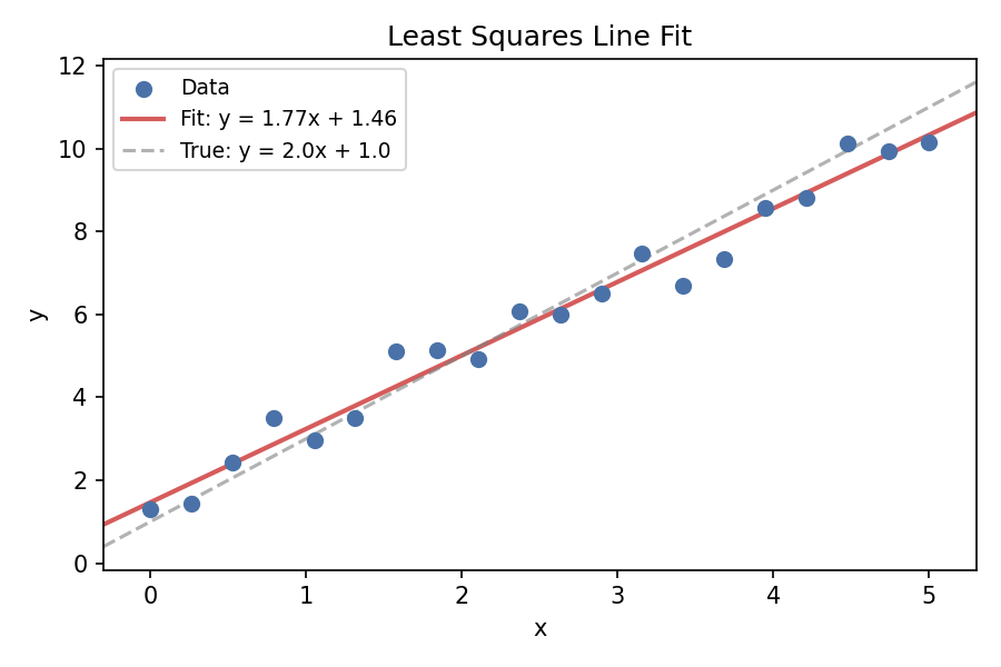
Given a set of points $(x_i, y_i)$, the simplest question in machine learning is: what line best describes them? The answer is a least squares fit: minimize the sum of squared vertical distances from the points to the line. This post walks through the math, the matrix form, and why QR is the right tool.
Problem Setup
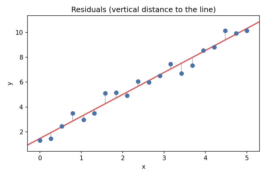
We are looking for a line $\hat{y} = mx + b$. For each observed point $(x_i, y_i)$, the error (residual) is $r_i = y_i - (m x_i + b)$. We want to minimize the sum of squared errors:
\[\min_{m, b} \sum_{i=1}^n (y_i - (m x_i + b))^2\]Write this in matrix form. Stack all $y_i$ into a vector, and all $x_i$ into a matrix with a column of ones for the bias:
\[\underbrace{\begin{bmatrix} y_1 \\ y_2 \\ \vdots \\ y_n \end{bmatrix}}_{y} = \underbrace{\begin{bmatrix} x_1 & 1 \\ x_2 & 1 \\ \vdots & \vdots \\ x_n & 1 \end{bmatrix}}_{X} \underbrace{\begin{bmatrix} m \\ b \end{bmatrix}}_{\theta}\]The loss becomes $L(\theta) = |X\theta - y|_2^2$, the squared Euclidean norm of the residual vector.
Minimizing the Error
Take the gradient of $L(\theta)$ and set it to zero:
\[\nabla_\theta L = 2 X^T (X\theta - y) = 0\]This gives the normal equations:
\[X^T X \theta = X^T y \quad \Longrightarrow \quad \theta = (X^T X)^{-1} X^T y\]Intuition: “We are projecting $y$ onto the column space of $X$. The residual $X\theta - y$ is orthogonal to every column of $X$: that is what $X^T (X\theta - y) = 0$ means. The solution is the point in $X$’s column space closest to $y$.”
The cost of forming $X^T X$ and solving is $O(n d^2 + d^3)$ where $d$ is the number of parameters (here $d = 2$). For small problems this is instant. But $X^T X$ squares the condition number: if $X$ is poorly conditioned, $X^T X$ is much worse.
For large problems ($n$ in the millions, $d$ in the thousands), even forming $X^T X$ is too expensive. Instead, use gradient descent: start from a random $\theta$, compute the gradient $\nabla_\theta L = 2 X^T (X\theta - y)$, step in the opposite direction, repeat. Each step costs $O(n d)$ instead of $O(n d^2 + d^3)$. The exact solution via normal equations or QR gives you the answer in one shot, but gradient descent scales to problems where one-shot methods do not fit in memory.
Modern Machine Learning problems are built around gradient descent, because numbers have gotten too large, but it is important to understand the exact solution they are approximating.
QR Is Better
Instead of the normal equations, use the QR decomposition from the previous post. Factor $X = QR$ where $Q \in \mathbb{R}^{n \times d}$ has orthonormal columns and $R \in \mathbb{R}^{d \times d}$ is upper triangular. Then:
\[\theta = (X^T X)^{-1} X^T y = (R^T Q^T Q R)^{-1} R^T Q^T y = (R^T R)^{-1} R^T Q^T y = R^{-1} Q^T y\]No squaring of the condition number, and solving $R\theta = Q^T y$ with back-substitution costs $O(d^2)$. QR is backward stable; the normal equations are not.
Intuition: “Normal equations compute $X^T X$, which squares the condition number (bad for ill-conditioned problems). QR works directly on $X$ and is stable. For a simple 2-parameter line fit the difference is academic, but for wide problems ($n \gg d$) the normal equations can lose digits to rounding.”
Beyond One Line
The same idea extends to multiple inputs and multiple outputs. Let each input be $x \in \mathbb{R}^i$ and each output be $y \in \mathbb{R}^o$. The linear model becomes:
\[y = W x + b, \qquad W \in \mathbb{R}^{o \times i}, \; b \in \mathbb{R}^o\]Each output is a linear combination of all inputs plus a bias. If you stack multiple inputs as rows of $X \in \mathbb{R}^{n \times i}$, the matrix form is $Y = X W^T + \mathbf{1} b^T$, and the least squares solution for $W$ and $b$ follows the same pattern.
This is a linear layer: one matrix multiply and one bias add, no activation. It is the simplest building block of a neural network.
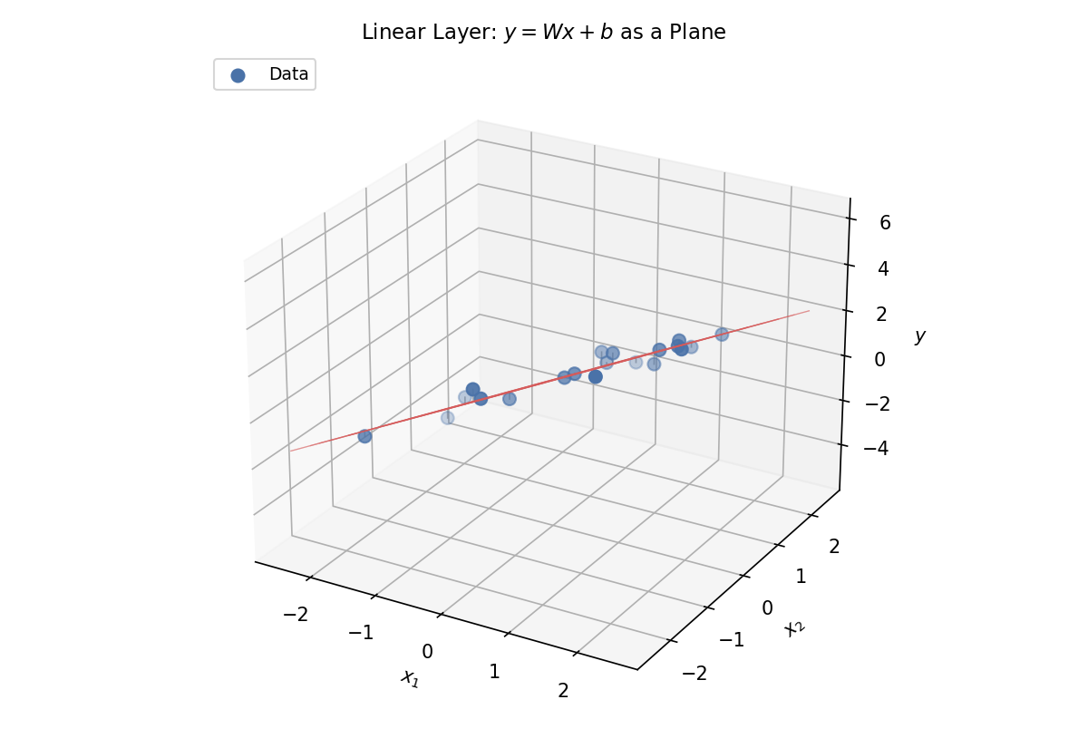
the line seems 1d from this angle, but it is actually a plane in 3D space. The concept of a best fit line, can be generalized to a best fit plane between points in 3d.
and then a best fit hyperplane between points in higher dimensions. And it can all be built by stacking linear layers on top of each other, and adding non-linear activations in between to break the linearity and turn lines into curves. That is the feed-forward network, the topic of the next post. This will be covered soon in a Feed Forward Networks post.
Intuition: “For one input and one output, the model is a line. For two inputs and one output, the model is a plane. For $i$ inputs and $o$ outputs, the model is a hyperplane in $(i + o)$-dimensional space: a linear mapping from input to output.”
Components
- $X \in \mathbb{R}^{n \times d}$: design matrix. Rows are data points, columns are features (plus a bias column of ones).
- $y \in \mathbb{R}^n$: observed outputs (targets).
- $\theta \in \mathbb{R}^d$: parameters (slope $m$ and intercept $b$ in the 1D case; all weights and biases in the multi-dimensional case).
- $L(\theta) = |X\theta - y|_2^2$: least squares loss. Minimizing this gives the maximum likelihood estimate under Gaussian noise.
- $\hat{y} = X\theta$: predictions: the orthogonal projection of $y$ onto the column space of $X$.
Quick Reference
| Aspect | Normal Equations | QR |
|---|---|---|
| Formula | $\theta = (X^T X)^{-1} X^T y$ | $\theta = R^{-1} Q^T y$ |
| Cost | $O(n d^2 + d^3)$ | $O(2 n d^2 - \frac{2}{3} d^3)$ |
| Stability | ❌ squares cond($X$) | ✅ backward stable |
| Use case | Small, well-conditioned | Ill-conditioned, production code |
Notes
- The normal equations are fine when $d$ is small and $X$ is well-conditioned. For anything else, use QR (or the SVD for rank-deficient problems).
- Adding a bias column of ones is equivalent to centering the data: subtract the mean of $x$ and $y$, fit $m$, then recover $b = \bar{y} - m \bar{x}$.
- The linear layer $y = Wx + b$ is the foundation of every neural network. The next post adds a non-linearity between layers to break the linearity and turn lines into curves: that is the feed-forward network.